A Novel Fibonacci Windows Model for Finding
Emerging Patterns over Online Data Stream
Tubagus M. Akhriza
School of Electronic Information and Electrical Engineering Shanghai Jiao Tong University
Shanghai, China [email protected]
Yinghua MA, Jianhua LI School of Information Security Shanghai Jiao Tong University
Shanghai, China
{ma-yinghua, lijh888}@sjtu.edu.cn
Abstract—Patterns i.e. the itemsets whose frequency increased significantly from one class to another are called emerging patterns (EP). Finding EP in a massive online data streaming is a tough yet complex task. On one hand the emergence of patterns must be examined at different time stamps since no one knows when the patterns may be emerging; on another hand, EP must be found in a given limited time and memory resources. In this work a novel method to accomplish such task is proposed. The history of itemsets and their support is kept in a novel data window model, called Fibonacci windows model, which shrinks a big number of data historical windows into a considerable much smaller number of windows. The emergence of itemsets being extracted from online transactions is examined directly with respect to the Fibonacci windows. Furthermore, as the historical windows are recorded, EP can be found both in online and offline mode.
Keywords—Emerging Patterns, Data Window Model, Online Data Stream
I. INTRODUCTION
In the era of information, massive data is being produced by almost every digital thing around the people. Social media and e-commerce generate and process the data continually while different kinds of computing devices and sensors receive it. On the other side, information possessed in the data is also evolving, such as the trend of patterns. Due to such fact, methods than can quickly discover the changing trend inside the online data stream are significantly needed. Concept of emerging patterns (EP) is usually used for this task. Given two classes of data, the patterns i.e. itemsets whose frequency increasing significantly from one class to another are called the emerging patterns and being the target in EP mining [1]. However, finding EP in online data stream faces several challenges. On one hand the emergence of patterns must be examined at different time stamps since no one knows when the patterns may be emerging. For example, to find an explosive growth of topics on news [2][3], an examination on short time topic is a must, but to find a mild prolonged growth, an examination on long time history is also a necessity [4]; on another hand, EP must be found in a given limited time and memory resources.
Literature studies found that the sliding window model is commonly used in finding EP over incremented datasets, like in these references [5–7]. A transaction window, Tr_window,
here, means a batch of transactions, and itemsets are mined from such Tr_window. This model is not fit to discover EP at different time stamps because patterns are examined only in between two Tr_windows: current and previous windows, while patterns found in the older Tr_windows are discarded.
This problem can be solved by keeping the history of itemsets and their supports for long term. Another model called logarithmic tilted-time windows (LTT-windows) model was proposed for finding frequent patterns (FP) at multiple time granularities, although it had never been applied in EP mining [8]. Given initially N batches of transactions, itemsets are mined from each batch and stored in an itemset window, It_window. Clearly, number of It_windows will be becoming bigger, as more batches are processed. LTT-windows model is proposed to pack the It_windows into high-compression-rate windows with smaller number. N number of It_windows will be packed into [1+log2(N)] number of LTT-windows. This model stores the supports in finer accuracy in some recent windows and coarser accuracy in the older LTT-windows. That is, an LTT-window merges a certain number of It_windows according to a sequence {1, {2n}} = {1, 1, 2, 4, etc.}. E.g. the 1-st and 2-nd LTT-window merges only one window i.e. the last one and last two most recent window. The 3-rd and 4-th LTT-window merges respectively two and four windows, and so on.
However this model cannot dynamically handle the online data streaming where transactions are coming continually and must be processed soon after their arrival, because when new transaction data comes, the computation need to be made to update data saved in LTT windows is too big to be handled online.
In this article, a novel method for finding EP over data stream both in online and offline mode is proposed using a new windows model called Fibonacci Windows (windows or F-Win) model. The purpose of F-windows development is similar with LTT-windows, but principally, Fibonacci sequence (shorted as Fibonacci) is used instead of 2n sequence. An F-window merges certain number of It_F-windows according to Fibonacci sequence. Every two F-wins are organized into one level. According to Fibonacci sequence (0, 1, 1, 2, 3, 5…), the first level {0, 1} accommodate at most one it_window, the second level {1, 2} accommodates at most 1 + 2 = 3 it_windows, the third level {3, 5} accommodates at most 8
it_windows, and so on, or generally, maximal number of windows accommodated at i-th level is
It_windows, where is the j-th element in Fibonacci. A new level will be created only if each lower level has reached its . This approach makes the Fibonacci windows model can flexibly and dynamically adjust to accumulating more It_windows.
An F-Windows system is created for each itemset. Following the Fibonacci sequence, the 1-st F-Window is always zero and the 2-nd F-Win will be containing the support of itemset being extracted by online. A session opened for online itemset extraction is called an online window. A maximum size of all itemsets generated in online window is limited to a user-given max_size threshold (in bytes); if it is reached, size counting is reset; at this time the current online window is “closed” and the new online window will be created. The closed windows are arranged in F-windows system explained above. The EP will then be inspected in between the 2-nd F-win and the other F-Wins. As a merit, since F-windows are recorded, EP can also be found in offline mode.
Experimental work was designed to demonstrate F-Windows system in finding EP at different time granularities. Two synthetic datasets with different items density were used in the experiment. The program for this experiment was developed so it is able to pop up the EP onto the console in real time. Experimental results discovered three types of EP based on their support growth: Once-emerging, seasonal-emerging and everlasting-emerging. These types are also defined for the first time in this article and also become a significance contribution of this work.
II. RELATED WORKS
Some current works related to EP mining are described in this section. As EP mining in incremented dataset is closely related to data windows models, some references regarding to the models are also explained.
A. Emerging Patterns Mining
Assume that we are given an ordered pair of datasets D and D . Set I contains all items in both datasets, and X I. Let sup X denotes support of X in D. Growth rate of X from D to D , denoted as GrowthRate(X), is defined as:
0 if sup X =0 and sup X =0 ∞ if sup X =0 and sup X ≠0 sup X
sup X otherwise
Given >1 as a growth-rate threshold, an itemset X is said to be an -EP (or simplify EP) from D to D if GrowthRate(X) ≥ , and the EP mining problem is, for a given growth-rate threshold , to find all -EP. In a special case when sup X = 0 and GrowthRate(X) ≥ , X is called Jumping EP (JEP) [1]. EP is a particular class of frequent itemsets [1]. An itemset X is called frequent in D , if sup X ≥ minsupp, a user-given minimum support threshold.
Mining FP over a big data stream is more complex than mining over static dataset. We have to cope with the
transactions which are streaming continually, rapidly and possibly in an unbounded size. The target application domains of a data stream are either a bulk addition of new transactions as in a data warehouse system or an individual addition of a continuously generated transaction as in a network monitoring system or web click stream. The former is called as an offline data stream while the latter is called as an online data stream [9]. However, rescanning big data is prohibitively expensive for both online and offline data stream [10]. The online data stream mining has purpose to give a quick answers for online queries about the patterns possessed in the streaming. Thus approximate solution (itemsets or supports) with reasonable loss are usually more acceptable [11] than the complete solution but sacrificing the time and memory resources. These considerations made the mining methods over data stream had some particular characteristics [9–11]. Each data element should be examined at most once to analyze a data stream. The memory usage for data stream analysis should be restricted finitely although new data elements are continuously generated in a data stream.
Finding EP in the streaming becomes much more complex since there is no clear bound between transactions in the streaming, whereas EP must be found in between two datasets. Some windows models were then used to bound the streaming data. In the following section these models are explain more detail.
B. Data Windows Model
There are mainly two data windows models proposed in mining patterns over incremented datasets: landmark windows model and sliding windows model [10]. Two other known models: damped window and tilted-time window models are basically the landmark window model with some improvements.
Landmark window model was proposed initially in [9][10][12] for finding FP in online data stream. Transactions are first collected into a “bucket” before processed. The bucket is later known as batch or window, or in this article, Tr_window. Tr_windows are processed at respective time stamps one after another, and the support of all itemsets is sum up from a Tr_window at a specific time stamp to current time stamp. This total summation made the transactions and the extracted itemsets are treated equally importance from time to time. For finding EP in incremented data, where the information about support found at different time stamps is needed, such plain landmark window model is clearly not fit. Further, some researchers also thought that the transactions are time-sensitive so they must not be treated equally by the time goes by. Due to such reason the other three models were proposed.
Damped window model is a landmark model with an improvement where an itemset has decay threshold associated with time [9][10][13]. The older the itemset, the less important is the itemset. As EP should be examined at any time stamp, this model does not work well because old itemsets will be disappeared after some periods gone by.
fixed time unit, e.g. one week, toward processing the most recent one week transactions while in the same time, the oldest one week transactions are discarded. The reason of such discarding is that they are not significant in showing the most recent trend changing. The major drawback of this model in finding EP is that the itemsets is examined only in between two Tr_windows: current and previous windows, and since we do not know the suitable length for the windows size and sliding unit, thus many EP could possibly be missed. This problem actually can be solved by keeping the history of itemsets’ supports found in old windows for long term. Literature studies found that the sliding windows model is commonly used in methods for finding EP from incremented datasets, and therefore these methods possessed the weakness of this model as explained above.
Another model called logarithmic tilted-time windows (LTT-Windows) model was proposed to store the history of itemset’s supports [8], although this model had never been applied in EP mining. This model basically is also a landmark model, because initially, a set of transactions must be divided into N batches. From each batch, itemsets are then extracted; their supports are calculated and stored into one It_window. Obviously, number of It_window for storing the itemset’s supports is big. LTT-windows were proposed to pack It_windows into smaller number. For initial N batches, the initial LTT-windows for an itemset X look like: s(n:n); s(n– 1:n–1); s(n–2; n–3); s(n – 4:n –7), …, where
: _
_
Sigma shows that the supports in those It_windows are merged. Number of It_windows merged into i-th LTT-window follows the i-th element in a sequence of {1, {2n}}, n ≥ 0 i.e. 1, 1, 2, 4, etc. LTT-windows show the idea of tilted-time windows []. The first two LTT-windows contain the finer accuracy of supports, because they are not resulted from merged supports, while the next LTT-windows provide the coarser accuracy as the supports are accumulated from merging process. This model shrinks N number of It_windows into [1+log2(N)] number of LTT-windows. However there are several shortcomings in LTT-windows model. N must be given in advance to reserve memory for the LTT-windows. Consequently, each itemset by default has [1+log2(N)] number of LTT-windows although it perhaps does not exist in the next processed batches. That is, at the initial process this model cannot dynamically handle the online data streaming where transactions are coming continually and must be processed soon after their arrival. This inflexibility causes the implementation of this model is somehow costly in online steaming environment. LTT-windows model was proposed initially to find FP in offline data stream, where bulky transactions were the target of the mining process [8].
III. PROPOSED METHODS
The problem of LTT-windows model is solved in our work by proposing a novel window model, i.e. the Fibonacci windows (F-windows) model so EP can be found in online data stream at different time stamps and time granularities. The sequence of {1, {2n}} in the former model is replaced with
Fibonacci sequence, or shorted as the Fibonacci: {0, 1, 1, 2, 3, etc.}. Finding EP at any time stamps in offline mode is also possible now since, F-windows are recorded. Before explaining the model and the algorithm for finding EP, this section explains the framework for finding EP over data stream.
A. Framework
As described, this work mainly aims to solve the problem of finding EP in online data stream, thus one-by-one transaction as its arrival is processed to extract itemsets from it. The transaction is discarded after processed, so Tr_windows are not needed. The itemsets extraction is performed in an online window, OL_window (or OL_win). As introduced earlier, OL_window actually does not exist physically and logically; instead, it is described as a session opened for online itemset extraction. The maximum size of itemsets in OL_win is limited to user-given max_size threshold, e.g. 1 MB. If the threshold is reached, the current OL_window is “closed” i.e. by resetting itemsets’ size counting to zero. The closed OL_windows are arranged in a novel window model proposed in this work, i.e. the Fibonacci windows model. Each itemset has its own F-windows which are also possibly different from the other itemsets because an itemset is not always found in every OL_window.
Right after an itemset is extracted in OL_window, its emergence is examined with respect to its records in the existing F-windows. On the other words, the purpose of online EP mining is to immediately check whether an itemset extracted in OL_window is an EP by comparing with history data saved in F-windows. As the model goes well in online data processing, let alone EP can also be found in offline mode. In offline mode, we have more relaxed time to explore more the F-windows and try more parameters to find EP. While in the online mode, being restricted to limited time the EP examination may be applied only on itemsets found and extracted into OL_window with certain predefined threshold.
B. Fibonacci Windows Model
The main design of windows is described in Fig. 1. An F-window (F-win) accommodates certain number of closed OL_windows according to the Fibonacci: {0, 1, 1, 2, 3, 5, etc.} by merging data saved inside OL_windows. F-win 1 and 2 respectively can accommodate data from none and one closed OL_window. F-win 3 and 4 respectively can accommodate one and two closed OL_windows, and so on. Every two F-wins, or a pair of F-Wins, are organized into one level. So the i-th level has its maximum accommodation capacity i.e.
, where is the j-th element in Fibonacci. For example, of 1-st level is (0+1) = 1, for 2-nd level is (1+2) = 3, and so on. On the other side, each F-win also has its
maximum value called and follows elements in
Fibonacci. Generally, F-win j’s = j-th element of Fibonacci.
F-wins in same level are stick together in respective squares. Rounded rectangle shows the updating path, while a separated rectangle is Lmax of a level.
Fig. 1. Fibonacci Windows Model Design
The updating works based on following basic rules: (1) F-win is either null or full, but it is not allowed to have
two null F-wins in a same level.
(2) F-win 2 is always filled and updated with the support of itemset being extracted in the opened OL_window.
(3) When new OL_window is created, a null F-win is searched from lower to upper level and from left to right in same level. The first null F-win i found in a level will be filled with F-Win (i-1) + F-Win (i-2), and the values of the merged Wins are set null. In this case, the first null F-win in the sequence will be the (i–1)-th F-win.
(4) While the first null F-win is not in the first level, merging operation described in step (3) will continue occur, until the first null F-win is F-Win 2 which is ready to accommodate the new created OL_window.
Fig. 2. Levels and F-wins Updating Mechanism
To make the updating process clear, the beginning of F-windows model is given in Figure 2. In Fig. 2(a) the first OL_Window is accommodated in F-Win 2 (as F-Win 1 is always full). When this first OL_window is going to close, as both wins in level 1 are full, they are merged and saved in F-Win 3, and F-F-Win 2 is prepared to accommodate the new OL_window, as shown in Fig. 2(b). Then before the next new OL_window is opened, F-Win 2 and 3 in Fig. 2(b) will be merged to F-Win 4, shown in Fig. 2(c). Next, since F-Win 3 is empty, it is ready to receive value from F-Win 2 while F-Win 2 will be filled up with OL_window, so now the sequence is 0, 1, 1, 2, which is again a Fibonacci (Fig. 2(d)). At this stage, all
levels reached their L so a new level will be created when new OL_window is created – as in Fig. 2(e).
In Fig. 2(g), a Fibonacci is thus constructed: 0, 1, 1, 2, 3. Updating process is principally similar with (b) step. First, F-Win 4 and 5 are merged and put in F-F-Win 6, thus F-F-Win 4 and 5 become null. Next, Win 2 and 3 are merged and put in F-Win 4, so F-F-Win 2 can accommodate the new created OL_window. Up to step (h), the sequence becomes 0, 1, 0, 2, 0, 5 (with two null F-win and four full F-wins).
For more detail steps needed in F-Windows updating, the following Algorithm 1 is given.
Algorithm 1: F-windows updating
1. Given F-wins with the first index is 1
2. L current highest level
3. If F-Wins do not generate Fibonacci
4. { // search the first null F-Win from bottom
5. m index of the first null F-Win found
6. // update F-wins
7. For (i = m, i > 2, m = m–2)
8. { F-Win(i) = F-win(i-1) + F-win(i-2) }
9. F-Win(2) = OL_win // finally update F-Win 2
10.} else {
11.If all wins generate Fibonacci, means, all F-Wins are full then:
12.F-wins.push_front(), create one new F-Win in front of F-Wins i.e. F-Win(1), and thus L will be added by 1
13.m 2L-1, index of the highest F-Win
14.For (i = m, i > 2, m = m–2){
15.F-Win(i) = F-win(i) + F-win(i-1)}
16.F-Win(2) = OL_win // finally update F-Win 2}
17.Stop
As described in Algorithm 1, one of two conditions will be found when updating F-Wins: all F-Wins do not generate or do generate Fibonacci. In the former condition, there is no creation of new F-Win (or level), while in the later one, a new F-Win must be created. See the difference of updating formulas for these two conditions in line 8 and 15 respectively. The push_front() method, such as in C++’s STL, creates a new Win in front of existing Wins and pushes them back, so F-Win(1) = null and F-Win(2) contains the previous F-F-Win(1) which is also null, while Win(2L–1) contains the previous F-Win(2L). Finally, F-Win(2) will be filled in with OL_win.
C. An Optional Progressive Updating Algorithm
Each time new OL-window is closed, F-wins would be updated to accommodate new data. The higher level the first null F-win is found, the higher the number of updating operation is. As shown in Fig.2 (g), two merging operations should be done because the first null F-win is found in level 3. That is, the number of merging operation which should be done to update the whole F-wins is the number of level in which the first null F-win is found minus 1.
summons the 5th level of F-windows which is accompanied by four merging operations. Even though, we can still be sure that the average number of merging operations is less than two.
Considering fast non-linear increment of Fibonacci number, huge number of OL_windows can be accommodated in F-Windows. As shown in Fig. 3 (right) an F-Windows system with 15 levels can accommodate 1,346,268 OL_windows. Supposed each OL_window saves data collected for one hour, 1,346,268 OL_windows store the data of more than 100 years. That means there is few chance we need to create F-Windows with more than 15 levels. Even though, in the calculation of big amount of data handled in windows, we still need to take care of the condition in which new level is appended, and at that time many merging operations have to be handled.
Fig. 3. Left: the i-th opened OL_Windows (axis) vs. Number of Merging Operations, Right: Number of OL_windows can be accommodated
In order to even the merging operations between the updating, and to meet the requirement of online data processing, an optional progressive algorithm is introduced here in which the shadows are used. Shadow is a companion F-win which is waiting for its position that currently being occupied by old win. Fig. 4 shows the procedure of F-windows grow to the 6th level. Using shadow, each time new OL_window is opened, at most two merging operations will be carried out, instead of finishing all the merging operations at one time. And updating progress will be accomplished in a bottom-up fashion.
Fig. 4. Shadow F-win which is used to even merging operations.
In Fig. 4(a), there were five merging operations should be done to update the F-window. Using shadow, we only accomplish two merging operations each time, hence, F-Win 1 and 2 are merged and so on F-Win 3 and 4. The new F-Win 5 (demonstrated as a round) has a shadow (square beneath new F-Win 5) in which old F-Win 5 existed, as shown in Fig. 4(b), while F-Win 1 to F-Win 5 are all updated with new data. F-win with new updated data is represented in italic font. So when there is only one merging operation, shadow will be merged to
its pair. As shown in Fig. 4(b) and (c), shadows merged with their pairs and generated new shadow in higher level. When there is no spare time to merge shadow, shadow stays, as Fig. 4(d) shown. Until in Fig. 4(e), shadow Win 9 merged with F-Win 10, and level 6 is appended as shown in Fig. 4(f).
D. EP Online and Offline Mining
Two modes for EP mining are explained in this section, where both of them implement the basic rules in updating the F-windows. In the online mode, the emergence, i.e. the GrowthRate of itemset X extracted into F-Win 2 is directly computed with respect to sup(X) recorded in the other F-Wins. In the offline mode, EP can be examined in between two of any existing level (or F-Win). However, the focus of experimental work will be only on the online mode.
Itemsets are extracted right after a transaction is received. As in online environment alphabetically sorting and re-indexing the item is costly, an item will be assigned by an integer index according to its first entrance to the item database. However, in this work not all itemsets are extracted from a transaction, but only those having length not longer than a given max_len threshold. This approach is taken because in online mode, the request about EP contained in the streaming must be answered quickly, thus itemsets whose support can grow faster are more preferable to be monitored. Obviously short itemsets are fit in such criterion, because many transactions can possibly contain them. Further, the infrequent itemsets may be becoming frequent and even emerging at any time stamp in the future. Because number of subsets of short itemsets that must be stored in the database becomes smaller as well, we are able to store them all and to report their change with the exact support.
Algorithm for itemset online extraction is given in Algorithm 2. X S is an itemset in S which is initially an empty set {}. Supposed items in transaction T = {a, b, c, d} are indexed, and given max_len = 3, then finally S = {a, b, ab, c, ac, bc, abc, d, ad, bd, abd, cd, acd, bcd}. The order of itemsets found by Algorithm 2 is shown in S. Line 8 demonstrates that X is stored in F-Win 2 with sup(X) is incremented accordingly.
Algorithm 2: Itemset Online Extraction
1. Input: Transaction T, max_len
2. Initialize: S = {}, X = {} S, Temp = {}
3. Read an item t in T
4. For each X in S
5. { X = X ∪ t // itemset X is generated here
6. If |X| ≤ max_len, Then
7. { Temp = Temp ∪ X
8. F_Win(2, [X, sup(X)++]) }
9. }
10. S = Temp; Temp={}
11.Continue step 3 for next item
Algorithm 3 is developed for finding the EP in online mode. Basically, it contains Algorithm 2 but after new itemset X is generated its emergence is evaluated through k-recent level. However, level can be replaced with F-Win if needed. Algorithm 4 for finding EP in offline mode is given afterward. In algorithm 3 and 4, itemset X is mined out as an EP if sup(X) ≥ minsupp and GrowthRate(X) ≥ .
Algorithm 3: Online Mode for EP Mining
1. Input: Transaction T, Minsupp ms, max_len, growthrate
2. Read an item t in T
3. Peform algorithm 1 to generate itemset X from t
4. For k=2 to X.level, k++
5. { A = Sup(X) in level k i.e. merge of two F-Wins in each level k
6. B = Sup(X) in F-Win 2
7. Calculate growthrate(X) = B/A
8. If growthrate(X)≥ and A ≥ ms then mine out X as EP in level k }
9. Continue step 2 for next item
Algorithm 4: Offline Mode for EP Mining
1. Input: F-windows, Minsupp ms, growthrate
2. Start_level = desired starting level
3. End_level = desired end level
4. Read an itemset X in start_level
5. For k=start_level+1 to end_level, k++
6. { A = sup(X) in end level
7. B = sup(X) in start_level
8. Calculate growthrate(X) = B/A
9. If growthrate(X)≥ and A ≥ ms then mine out X as EP in between start level and level k }
10. Continue step 4 for next itemset
IV. EXPERIMENTAL WORKS AND DISCUSSION
A. Experimental Setting and Dataset
The aim of the experiment was to demonstrate the flexibility of F-Windows system in handling online EP mining at different time granularities. To this aim, the implementation of algorithms is explained as follows.
As there was no prior knowledge about the itemset supports and numbers, the setting of max_size, minsupp, and thresholds depends on the item’s density of the dataset. The higher the density, the bigger the thresholds is. When the support of an itemset X found in OL_win was being saved into F-Win 2, it was also directly compared with its previous sup(X) recorded in F-Wins in level 2 i.e. F-Win 3 and F-Win 4, as well as the highest F-Win. All JEPs and EPs were shown on the screen, and all those processes were done in real time. Information about the last OL_window that produced X was also displayed. The complete information shown on the console is like the following:
Two transaction datasets T1 and T2 used in the experiment were synthetic and generated using IBM Quest dataset generator program. The first one contains less density items (1:115 = item: transactions) and the second one has higher density (1:57). Average length of pattern was three with the correlation and confidence of items was 0.25 and 0.75 respectively. These settings were given as the default by the program.
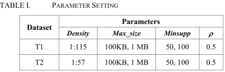
Parameters’ setting for experiments is given in table 1. Max_len = 3 was applied for both transactions. Each dataset was processed in 60 minutes of streaming. Smaller minsupp was used to keep more itemsets in F-wins, while larger max_size made each F-win can accommodate all EPs.
TABLE I. PARAMETER SETTING
Dataset Parameters
Density Max_size Minsupp
T1 1:115 100KB, 1 MB 50, 100 0.5
T2 1:57 100KB, 1 MB 50, 100 0.5
The framework was developed using VC++ Express edition 2013 with standard template library (STL) and run under Windows 7 32-bit on a PC with Intel Core i5 CPU, 650 @3.20 GHz and 3.33 GHz, with RAM 2 GB.
B. Results and Discussions
The first experiment used T1 i.e. the less density dataset as the input with max_size = 100 KB and minsupp = 50. As the output, 24 itemsets were popped up at the first time, i.e. as JEP, onto the console when the 2-rd OL_window was being opened and two of them had their support increased in the next OL_window such as shown below.
3018 : 34 1339 : 27 F-Win 3: 0 Growth: 1.#J F-Win 3: 0 Growth: 1.#J F-Win 4:51 Growth: 0.529 F-Win 4:62 Growth: 0.548 Highest: 51 Growth: 0.529 Highest: 62 Growth: 0.548 Last OL Win: 3 Last OL Win: 3
Interestingly, sup(X) in F-Win 3s was zero so the GrowthRate(X) was calculated with sup(X) in F-Win 4s. This was because when three OL-windows were (or being) processed, the Fibonacci sequence generated by the proposed method is 0, 1, 0, 2 and thus sup(X) is F-Win 3 was zero. On the other side, because F-Win 4 was the highest F-Win thus sup(X) in the Highest and F-Win 4 had a same value.
When the 7-th OL_window was being opened, there were 30 more JEPs popped up. But not all of them had support in F-Win 3 or F-F-Win 4 because their support had no increment after 5-th OL_window was closed. The absence of sup(X) in F-Win 3 was because sup(X) < 50. Support varied hugely, but when F-wins accumulated, the highest F-win (with biggest number of transactions saved inside) approached the real distribution of all itemsets.
Results from experiment on T1 using minsupp = 50 and on T2 using minsupp = 100 are provided in Fig. 5 and 6 respectively. The other results using different parameters are explained by referring to these figures.
In the experiment on T1, different max_size was used. When using max_size = 100 KB, while minsupp = 50, there were 33 OL_windows and 8,528 transactions were processed with 597 itemsets were popped up as the EP after 60 minutes passed. In amount of 557 itemsets among of them were JEP.
When using max_size = 1 MB, there are some significance differences shown on chart in Fig. 5. Number of OL-windows reduced to only five. More than 30 JEPs were popped up in the Itemset X : sup(X)
1-st OL_win. Smaller numbers of OL_windows was, the time consumption for updating the F-windows in the itemsets became shorter, more transactions were saved in F-windows. Specifically, 11,439 transactions were saved using max_size 1 MB, and more EPs i.e. 683 itemsets including 318 JEPs were found. Compared with the previous experiment (40 EPs), number of EPs in this experiment is much bigger.
Fig. 5. Chart of experiment on T1 using minsupp = 50
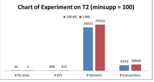
Obviously, the result showed that the size of F-win should be big enough to avoid splitting data in different windows which lead to losing relationship of data. Same result can also be gotten in experiment on T2 (shown in Fig. 6). In the experiment on T2, using max_size = 100 KB and minsupp = 100, there were 34 OL_windows were created, while using max_size = 1 MB, number of OL_windows created was four. Among data, with bigger max_size, more EPs were found, and more transactions were accommodated (support higher than minsupp).
But on the other hand, too big F-win slowed down creation of new F-win, which led to big delay when finding EPs by comparing the support in different F-wins.
Fig. 6. Chart of experiment on T2 using minsupp = 100
Nevertheless, there are some other remarkable notes gotten from the observation of experimental results. For example in the experiment on T1 using minsupp = 50 and max_size = 100 KB. The smallest support of EP was 50, which equals 0.5% with respect to 8,528 numbers of processed transactions, and this support is considerable as a very low support. As data are isolated in different OL_windows, many itemsets were not found in some F-wins because of low support inside, but still
they can be found in other F-Win, especially the (very) old ones, which holds the biggest accumulation of support recorded. These facts tell that itemsets must be given a chance to be emerging in the future by keeping them for a quite long term, as they can be emerging at any time points. Clearly, this is a significance advantage of the proposed approach which is not provided in sliding windows model where the oldest transactions and itemsets will be discarded.
Compared to LTT-windows, the F-Windows model also possesses some advantages. New F-Wins are created only when all F-Wins generated Fibonacci, while a fixed number of LTT-window is created in advance for all itemset. This shows the flexibility of F-Windows in handling online data stream where the presence of itemsets is uncertain in the transactions.
Another merit of F-Windows is that EP can be discovered in real time not only in between the OL_win i.e. F-Win 2 and F-Win 3, but also the other F-Wins. We can also know the last OL_win(s) in which the itemsets were found, so we have knowledge about how new is the itemset and when it became emerging last time. As shown in the first experiment, some itemsets’ support was stopped increasing at the 5-th OL_win, while the 20-th OL window is currently being opened.
In another case, we also found that some itemsets were stopped increasing for a while, before they started to increase again. This fact shows that some itemsets are probably emerging seasonally. Another interesting phenomenon was also captured in experiment on T1 that all 41 itemsets’ supports were increasing again at the 30-th OL_win, after their supports were all stagnant for some periods.
From such observation, an important summary is drawn in this article. Three types of emerging patterns based on their support growth in online data stream are discovered from the experiment:
(1) Once-Emerging – the itemset which only emerged once in an OL_window and its support never increased afterward. (2) Seasonal-Emerging – the itemset which was emerging in
one (or more) OL_windows, but it was absence for some certain time points before it is re-emerging in current OL_window.
(3) Everlasting-Emerging – the itemset which its support increasing continually in (almost) all OL_windows since its emerging for the first time.
In the real world these types of EP eventually appear. A topic in news might be emerging suddenly, but then fading out after some days passed. Name of particular sports wears or clubs might be emerging during some particular events or seasons. On the other side, some digital gadgets are known to be constantly popular since its first appearance, or also IT based skills which are mostly needed by the industries and almost always mentioned in job ads. The two latter examples are of the third type of EP defined above.
relatively much smaller number of F-Windows. The experimental work shows that this model is fit to find EP in real time over streaming datasets. Some parameters are adjustable to meet the characteristic of dataset density. Finally, three types of emerging patterns based on their support growth in online data stream were defined for the first time in this work.
Further, it is observed that length of emerging itemsets is also growing, which indicates that the dependency between itemsets is also changing and emerging. Finding the emerging dependency between itemsets is important for certain circumstances. For example, finding immediately the new unpopular IT skills, which are needed by industries and must be taught together with the known and popular skills set, is significance to improve teaching syllabi in a school. Therefore, the emerging dependency between itemsets will be focused on our future research.
ACKNOWLEDGMENT
This work is funded by the National Natural Science Foundation of China under grant No.61171173 61271316, and by Science and Technology Commission of Shanghai Municipality (14DZ1104903). This work is also supported by Chinese National Engineering Laboratory for Information Content Analysis Technology and Shanghai Key Laboratory of Integrated Administration Technologies for Information Security.
REFERENCES
[1] G. Dong and J. Li. “Efficient mining of emerging patterns: discovering trends and differences,” KDD, ACM International Conference on, 43-52, 1999
[2] A. Rudat and J. Buder. “Making retweeting social: the influence of content and context information on sharing news in Twitter,” Computers in Human Behavior 46 (2015) 75–84
[3] Saleem, H.M., Xu, Y., and Ruths, D. “Novel situational information in mass emergencies: what does Twitter provide,” Procedia Engineering 78 ( 2014 ) 155 – 164.
[4] H. Li, S. Lee and M. Shan . “An efficient algorithm for mining frequent itemsets over the entire history of data streams,” First international workshop on knowledge discovery in data streams, in conjunction with the 15th European conference on machine learning ECML and the 8th European conference on the principals and practice of knowledge discovery in databases PKDD, Pisa, Italy, 2004
[5] M. S. Khan, F. Coenen, D. Reid, R. Patel, and L. Archer. “A sliding windows based dual support framework for discovering emerging trends from temporal data,” Knowledge-based System, International Journal on, Vol. 10,316 – 322, 2010
[6] C. Lee, C. Lin and M. Chen. “Sliding-window filtering: an efficient algorithm for incremental mining,” Information and knowledge management (CIKM), ACM International conference on, 263–270, 2001 [7] J.H. Chang and W.S. Lee. “estWin: Online data stream mining of recent frequent itemsets by sliding window method,” Information Science, Journal of, Vol. 31, No. 2, 76–90, 2005
[8] C. Giannella, J. Han, J. Pei, X. Yan, and P. Yu. “Mining frequent patterns in data streams at multiple time granularities,” In: H. Kargupta, A. Joshi, D. Sivakumar, Y. Yesha (eds) Data mining: next generation challenges and future directions, MIT/AAAI Press, pp 191–212, 2004 [9] J. Cheng, Y Ke, and W. Ng. “A survey on algorithms for mining
frequent itemsets over data streams.” Knowl Inf Syst, Journal of, Vol. 16, 1–27, 2008
[10] V.E. Lee, R. Jin and G. Agrawal. “Frequent pattern mining in data streams,” in Frequent Pattern Mining, C. C. Aggarwal, J. Han (eds.), 199 – 224, Springer International Publishing Switzerland, 2014
[11] N. Jiang and Le Gruenwald. “Research issues in data stream association rule mining,” SIGMOD Record, Vol. 35, No. 1, 14–16, 2006
[12] G.S. Manku and R, Motwani. “Approximate frequency counts over data streams,” 28th international conference on very large data bases, Hong Kong, August, 346–357, 2002