A DYNAMICAL SYSTEM APPROACH IN MODELING TECHNOLOGY TRANSFER | Husniah | Journal of the Indonesian Mathematical Society 212 623 1 PB

(1)

Vol. 22, No. 1 (2016), pp. 37–59.

A DYNAMICAL SYSTEM APPROACH IN MODELING

TECHNOLOGY TRANSFER

Hennie Husniah

1

, Sebrina

2

and A.K. Supriatna

3

1

Department of Industrial Engineering, Langlangbuana University, Bandung 40261, Indonesia

email: hennie.husniah@gmail.com 2

PT Chevron Pacific Indonesia Rumbai, Pekanbaru, Riau 28271, Indonesia

email: sebrinafrey@gmail.com 3

Department of Mathematics, Padjadjaran University, Jatinangor 45363, Indonesia

email: a.k.supriatna@unpad.ac.id

Abstract. In this paper we discuss a mathematical model of two parties technol-ogy transfer from a leader to a follower. The model is reconstructed via dynamical system approach from a known standard Raz and Assa model and we found some im-portant conclusion which have not been discussed in the original model. The model assumes that in the absence of technology transfer from a leader to a follower, both the leader and the follower have a capability to grow independently with a known upper limit of the development. We obtain a rich mathematical structure of the steady state solution of the model. We discuss a special situation in which the upper limit of the technological development of the follower is higher than that of the leader, but the leader has started earlier than the follower in implementing the technology. In this case we show a paradox stating that the follower is unable to reach its original upper limit of the technological development could appear when-ever the transfer rate is sufficiently high. We propose a new ‘paradox-free’ model to increase realism so that any technological transfer rate could only has a positive effect in accelerating the rate of growth of the follower in reaching its original upper limit of the development.

Key words and Phrases: Dynamical system, technology transfer, knowledge man-agement, logistic curve.

2000 Mathematics Subject Classification: 90B70, 37N40, 97M50. Received: 04-07-2015, revised: 23-03-2016, accepted: 26-03-2016.

(2)

H. Husniah,

Abstrak.Di dalam makalah ini dibahas sebuah model matematika mengenai trans-fer teknologi dari seorang individu atau suatu parti yang disebutleader kepada seorang individu atau suatu parti yang disebutfollower. Model tersebut direkon-struksi melalui pendekatan sistem dinamik dari model standar Raz-Assa yang sudah dikenal. Hasil analisis model memperlihatkan sebuah sifat dari model hasil rekon-struksi yang tidak ada dalam bahasan model aslinya. Model Raz-Assa mengasum-sikan bahwa ketika tidak ada transfer teknologi, masing-masing individu atau parti mempunyai kapasitas untuk berkembang secara independen menuju batas atas yang diketahui. Selain itu juga diperlihatkan sifat-sifat solusi setimbang dari model terse-but di atas. Kemudian juga dibahas situasi khusus di manafollower mempunyai batas atas perkembangan yang lebih tinggi dibandingkan denganleader, namun ter-lambat dalam implementasi teknologi terkait dibandingkan denganleadertersebut. Dalam situasi seperti ini akan diperlihatkan suatu paradox di manafollowertidak akan pernah mencapai batas atas kapasitasnya apabila laju transfer teknologi terlalu tinggi. Untuk mengatasi paradox ini sebuah model baru diperkenalkan, sehingga laju transfer teknologi selalu memberikan efek positif terhadapfollower dalam hal pencapaian batas atas pengembangan teknologinya.

Kata kunci: Sistem dinamik, Transfer Teknologi, Manajemen Ilmu, Kurva Logistik

1. Introduction

Technology transfer has been defined as a process of the implementation of scientific/technological information developed in one area into another area, or equivalently defined as a process of migration and redeployment of technology from one area into different area [2, 18, 22]. The transfer could be done either by a mar-ket oriented mechanism, e.g. purchasing, licensing, etc., or a non marmar-ket oriented mechanism, e.g. academic journal, industrial fair, etc. [16]. Three main compo-nents in the process of technology transfer are the technology, the owner of the technology (also called as a leader, transferor, or donor), and the recepient (also called as a follower, transferee, or receiver). The process is usually complex involv-ing many related aspects, such as the properties of the technology beinvolv-ing transfered, the transferor capability of tranferring, and the transferee capability of adapting the technology [4, 14].

One important thing of technology transfer is the assesment of the future and the long-term behaviour of the technology transfer, which is known as techno-logical forecasting [26]. There are many literatures discussing this important, yet complicated, area of research. In general, mathematical modeling has been widely accepted as one approach in attacking complicated problems in many areas of in-dustrial engineering research (e.g. [6, 7, 9, 8, 1, 17]). However, despite numerous works on technology transfer, to date the use of mathematical modeling in this area is still limited. Among the known literatures on technology transfer that uti-lize mathematical models are [5, 10, 15, 19, 20, 23]. These models, and also related models regarding technological diffusion, e.g. [21], have been critically reviewed in [16].

(3)

technology gap between the transferor and the transferee, and the function gov-erning the technology transfer rate are used to develop the model for investigating technology transfer which relates to the behaviours of the technological leader and followers. In general, the model of the technological follower consists of two contri-butions, those from indigenous development indicating by the indigenous ability to develop (kF) and those from the interaction between the technology transfer rate (kT) and the technology gap between the leader and the follower. The general form of the model is given by

dXF(t)

dt =kFf0(XF(t)) +kTf1(XF(t))f2(XF(t), XL(t)). (1)

HereXF(t) is a measure of technological development for the follower and usually in the form of logistic growth (it is also called sigmoid, S-type growth, a growth with saturation [13]), or Gompertz-type growth [24].

In this paper we reconstruct and paraphrasing the model in [19], which is a special form of equation (1), via dynamical system approach [25]. This approach is similar to system dynamics approach proposed by Jay Forrester [3] and among the best framework available in predicting the long-term behaviour of the solution of dynamic systems, such the case in technology transfer. Recently, system dynamic approach has been used in addressing technological forecasting problems, since it can enhance insight in the essence of the problems by allowing the development of more complex model to investigate the structures and to further focus on the processes of the underlying technological forecasting aspect [11].

We found some important hidden notions of technological transfer arising from the model of Raz and Assa [19], which have not been discussed in their original paper. For example, we show a paradox stating that ‘the follower is unable to reach its original upper limit of the technological development could appear whenever the transfer rate is sufficiently high’. This is caused by an implicit assumption that there might be a negative effect of technology transfer whenever the transferee has a significant ability to develop in the absence of technology transfer. We propose a new model of technology transfer by modifying those in [19], which appropriately fits to reflect a technology transfer in which the transferee has a significant ability to develop in the absence of technology transfer. In this new model we assume that the presence of technology transfer from the transferor always has a positive effect in the technology development of the transferee. The model has a wide spectrum of application as long as we provide appropriate measurement to the level of development of the technology under consideration.

2. Raz and Assa Coupled Logistic Model

(4)

H. Husniah,

and for the follower is given by

XF(t) =

uF 1 +bFe−KFt

, (3)

wherebL andbF are constants and:

uL - is the upper limit of the technological development of the leader,

uF - is the upper limit of the technological development of the follower,

kL - is the indigenous ability of the leader to develop,

kF - is the indigenous ability of the follower to develop.

In this model, without any technology transfer from the leader, equation (3) tells us that the follower could attain the maximum level of the technology development by solely use of its indigenous ability to develop. In the presence of technology transfer, their model (equations (5) and (10) in [19]) takes the form

XL(t) =

. It is easy to check that the right hand side of equation (4) is the solution of the logistic differential equation

dXL(t) at t = 0. Consequently, equation (4) can be replaced by equation (6). Note also that gF in equation (5) is actually the growth rate of the follower development in the absence of technology transfer, that isgF = _dtd

_u similar argument as in the case of the leader,gFin equation (5) can also be replaced by dX˜F(t)

. Hence, the system (4-5) can be rewritten in the form

(5)

Proposition 2.1. The system of equations (7) and (8) has four steady state solu-tions with exactly one positive steady state solution.

Proof. The steady state solutions of equations (7) and (8) are obtained by equat-ing both equations to zero and solve forXL andXF. The system has four steady states, namely (X∗

F2 and XF∗3 ensure that there is a non-trivial steady state. Further-more, since the product of the roots is negative then there is exactly one positive

non-trivial steady state.

The proof in the proposition shows that the indigenous ability of the leader to develop (kL) does not appear in the steady state. This means that the level of the technological development of the follower is independent from the indige-nous ability of the leader to develop. However, the upper limit of the technological development of the leader (uL) and the rate of technology transfer (kT) critically affect the technological development of the follower with the structural properties described in Propositions 2.1 to 2.4.

Proposition 2.2. The positive steady state solution (X∗

L2, XF∗2) = (uL, Z1∗) is stable while all other steady states are unstable.

Proof. The stability of a steady state is determined by the negative sign of all the eigenvalues of the associated Jacobian matrix.

(1) The eigen values of the Jacobian matrix for (X∗

L0, XF∗0) arekLandkF−kT, which is not all negative.

L1, XF∗1) arekLandkT−kF, which is not all negative.

L2, XF∗2) are −kL and

L3, XF∗3) are −kL and

Proposition 2.3. The stable steady state solution (X∗

L2, XF∗2) has the following properties:

(6)

H. Husniah,

(a) First we prove the left part of the inequality in the general case,

X∗

Next we prove the right part of the inequality as follows,

X∗

(b) Here we only prove the left part of the inequality in the casekF > kT since the right part is the same as above.

(7)

(a) First we prove the left part of the inequality in the general case,

Next we prove the right part of the inequality as follows,

X∗

(b) Here we only prove the right part of the inequality in the case of

kF < kT since the left part is the same as above.

(8)

H. Husniah,

the maximum leveluF eventually, regardless the technological development level of the leader. However, in the presence of technological transfer, Propositions 2.1-2.3 show this is true only ifuF =uL. In this case there is a trade-off among the leader and follower parameters. The Proposition 2.4 uncovers more results regarding the trade-off for some spesific parameters.

On the other hand we also have

(9)

(3)

X∗

F2 =

muL(nkT−kT) +

p

(muL(nkT−kT))2+ 4nkTkTmuLuL 2kF

< n(n−1)kTuL+

p

(n(n−1)kTuL)2+ 4nn(kTuL)2 2kF

= (n(n−1) +n(n+ 1))kTuL 2nkT

=nuL.

On the other hand we also have

X∗

F2 =

muL(nkT −kT) +

p

(muL(nkT −kT))2+ 4nkTkTmuLuL 2kF

,

> m(m−1)kTuL+

p

(m(m−1)kTuL)2+ 4mm(kTuL)2 2kF

,

= (m(m−1) +m(m+ 1))kTuL 2mkT

= (m

n)uL.

(4) It is clear from result (1) of the proposition. (5) It is clear from the definition ofX∗

F2.

Note that Proposition 2.4 implies the maximum level of the follower technological development is given byX∗

F2≤max(uF, uL). In the next section we presents some examples to illustrate the results described in the propositions.

Raz-Assa Model foruF < uL withkT = 0.0

Figure 1. Plots ofXL(t) (solid),XF(t) (dash), andXL(t)₋XF(t) (dots) withuF = 1,

(10)

H. Husniah,

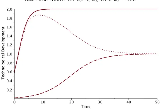
Raz-Assa Model foruF < uL withkT = 0.3

uL= 2,kT = 0.3.

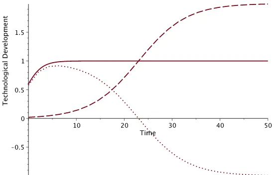
2.1. Numerical Examples of Raz and Assa Coupled Logistic Model. Fig-ure 1 shows the plots of the leader technological development XL (solid) and the follower technological developmentXF (dash) with respect to time, as the solution of equations (7) and (8), respectively. Dots represent the technological gap between the leader and the follower. The parameters used in this example are taken from [19] (except that kT = 0), i.e. kL = 0.6,kF = 0.2,uL = 2,uf = 1 with the initial states of the technological development are XL(0) = 0.6 and XF(0) = 0.02. Fig-ure 2 shows the solution to the same situation but in this case there is a transfer technology from the leader to the follower with kT = 0.3. Note that the max-imum technological development of the follower is now above its original upper limit (uF=1 andXF∗2is about 1.5) due to the presence of the technology transfer. Next we assume the following situation. Both parties, sayLandF, develop a certain technology independently, with the same parameters as above, except the values ofuL anduF are reversed, i.e.,uL= 1 anduF = 2, and they begin from the same initial condition, i.e. XL(0) =XF(0) = 0.02. The solution to this problem in the absence of technology transfer is illustrated by Figure 3. Furthermore, if

L is heading in this technological contest compared to L, e.g. XL(0) = 0.6 and

XF(0) = 0.02, then we have Figure 4 as the illustration. Next suppose that since

(11)

presence of technology transfer together with the gap of technological development affect the follower rate of development.

Raz-Assa Model foruF > uL withkT = 0.0 [the same initial conditions]

uL= 1,kT = 0.

Raz-Assa Model foruF > uL withkT = 0.0 [different initial conditions]

(12)

H. Husniah,

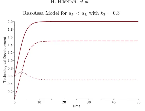
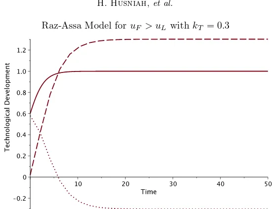
Raz-Assa Model foruF > uL withkT = 0.3

uL= 1,kT= 0.3. The case where the paradox of technology transfer occurs.

3. Modification of the Raz and Assa Coupled Logistic Model

3.1. The First Modified Model. The first revision to the model is done by assuming that the presence of technology transfer affects the follower’s ability to develop kF. Hence the model is given by equations (9) and (10) with the results presented in Propositions 3.1.1-3.1.2.

dXL(t)

dt =kLXL(t)

1−XL(t)

uL

, (9)

dXF(t)

dt = (1 +kT(XL(t)−XF(t)))kFXF(t)

1−XF(t)

uF

, (10)

Proposition 3.1. The system of equations (9) and (10) has six steady state solu-tions with exactly two positive co-existence steady state solution.

Proof. It is clear that by equating both equations (9) and (10) to zero and solve for

xL andxF we found six steady states, namely (XL∗0, XF∗0) = (0,0), (XL∗1, XF∗1) = (0, uF), (XL∗2, XF∗2) = (0,1/kT), (XL∗3, XF∗3) = (uL,0), (XL∗4, XF∗4) = (uL, uF), and (X∗

L5, XF∗5) = (uL,1+k_kT_TuL). This completes the proof.

L4, XF∗4) = (uL, uF) is stable and (X∗

(13)

Proof.

L0, XF∗0) are kL and kF, which is all positive.

L1, XF∗1) arekLandkF(kTuF− 1), which is not all negative.

L2, XF∗2) arekLand

kF(kTuF₋1)

kTuF , which is not all negative.

L3, XF∗3) are−kLandkF(1+

ktuL), which is not all negative.

L4, XF∗4) are−kLand−kF−

kFkTuL+kFkTuF. Note that −kF −kFkTuL+kFkTuF =kF(kT(uF −

uL)−1) =kF(T0−1), hence it is negative wheneverT0<1, means that the steady state is stable. Otherwise, ifT0>1 then the eigen value is positive, means that the steady state is unstable.

L5, XF∗5) are−kLandλ42=

means that this steady state is unstable. Meanwhile, in the case of T0>1 we have

means that this steady state is stable.

(14)

H. Husniah,

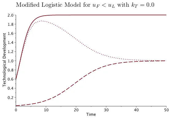
Modified Logistic Model foruF < uLwith kT = 0.0

uL= 2,kT = 0.

Modified Logistic Model foruF < uLwith kT = 0.3

uL= 2,kT = 0.3.

Figure 6 shows the plots of the leader technological developmentXL (solid) and the follower technological developmentXF (dash) with respect to time, as the solution of equations (9) and (10), respectively. Dots represent the technological gap between the leader and the follower. As before, the parameters used in this example are taken from [19] (except that kT = 0), i.e. kL= 0.6,kF = 0.2,uL= 2,

(15)

and XF(0) = 0.02. Figure 7 shows the solution to the same situation but in this case there is a transfer technology from the leader to the follower with kT = 0.3. Note that the maximum technological development of the follower is the same as before, i.e. X∗

F2=uF = 1, but it is reached relatively faster than in the absence of technology transfer.

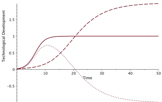
Next we assume the following situation. Both parties, sayLandF, develop a certain technology independently, with the same parameters as above, except the values of uL and uF are reversed, i.e., uL = 1 and uF = 2, and they begin to develop from the same initial condition, i.e. XL(0) = XF(0) = 0.02. The solution to this problem in the absence of technology transfer is illustrated by Figure 8. Furthermore, if L is heading in this technological contest compared to

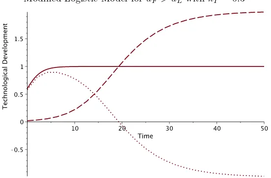
L, e.g. XL(0) = 0.6 andXF(0) = 0.02, then we have Figure 9 as the illustration. Next suppose that since F is lagged behind, in terms of the innitiation of the technological implementation, and there is a transfer technology fromLtoF with

kT = 0.3, then the development of technology of the two parties is depicted by Figure 10. Different from prediction derived by the original model, in which the follower cannot attain its original upper limit of technological developmentuF, here

uF can be attained in a faster time (Figure 10) compared to the time needed in the absence of technology transfer (Figure 9). Figure 10 also illustrates the stability of

uF sinceT0= 0.3<1 (see Proposition 3.2 and also Figures 11 and 12).

Modified Logistic Model foruF > uL withkT = 0.0 [the same initial conditions]

uL= 1,kT = 0.

Note that by referring to the proof of Proposition 3.2, there is a switching of stability between (X∗

L4, XF∗4) and (XL∗5, XF∗5) depending on the value ofT0, hence the value T0 = kT(uF −uL) is a stability threshold. The figures show that in a

(16)

H. Husniah,

Modified Logistic Model foruF > uL withkT = 0.0 [different initial conditions]

uL= 1,kT = 0.

Modified Logistic Model foruF > uLwith kT = 0.3

uL= 1,kT= 0.3. In this case the thresholdT0= 0.3<1, hence (uL,uF) is stable.

(17)

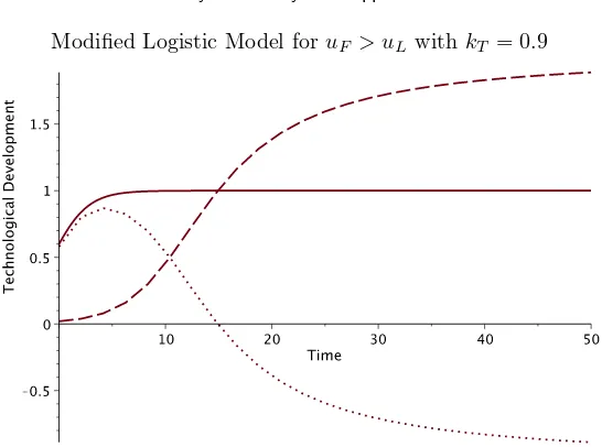
Modified Logistic Model foruF > uLwith kT = 0.9

uL= 1,kT= 0.9. In this case the thresholdT0= 0.9<1, hence (uL,uF) is stable,

although it looks unstable. See Figure 12 for the long-term behaviour.

Modified Logistic Model foruF > uL withkT = 0.9 [the long-term behaviour]

uL= 1,kT= 0.9 beyond 100 time course. It is clear, since the thresholdT0= 0.9<1,

the equilibrium state (uL,uF) is stable.

(18)

H. Husniah,

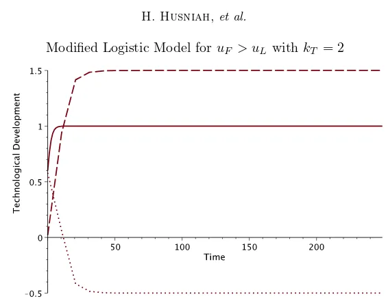
Modified Logistic Model foruF > uL withkT = 2

uL= 1,kT = 2. It is clear, since the thresholdT0= 2>1, the equilibrium state (uL,uF)

is unstable. In this case the stable equilibrium state is (uL,1+ k_Tu_L

kT ) indicating the

occurence of the technology transfer paradox.

Max-ML Model foruF > uL withkT = 2

Figure 14. Trajectories of system 11 and 12 for three different transfer rates, i.e. kT = 2,0.3 and 0.0, together withuF = 2 anduL= 1 (the other parameters are the

same as in the previous examples). As it is expected the model gives a paradox-free result, in which technology transfer always enhances the growth of the follower.

(19)

3.3. The Second Modified Model. Here we assume that the presence of tech-nology transfer explicitly has a non-negative impact in increasing the follower’s rate of development. We call the model as the Maximum Modified Logistic (Max-ML) model with the governing equations given as follows,

dXL(t)

The following propositions are the main results of the model’s behaviour in terms of its equilibria. The propositions will show that the model rectifies/removes the occurence of the unwanted paradox appearing in the earlier models.

Proposition 3.3. The system of equations (11) and (12) has six steady state so-lutions with exactly two positive co-existence steady state soso-lutions.

Proof. It is clear that by equating equation (11) to zero and solve for XL we found two solutions, namely X∗

L = 0 and XL∗ = uL. To find the steady state

= 0. We solve this equation forXF, by looking at the following two cases, namelyX∗ 0, hence we obtain three solutions, X∗

F = 0, XF∗ = uF, and one solution from (1 + max(0, kT(−XF(t)))) = 0 which exists when max(0, kT(−XF(t))) = −kTXF(t) and satisfied by XF∗ = k1T. Consequently, the steady state solutions for the system in this case are: (X∗

L0, XF∗0) = (0,0), (XL∗1, XF∗1) =

kT . Consequently, the steady state solutions for the system in this case are: (X∗

L3, XF∗3) = (uL,0), (XL∗4, XF∗4) = (uL, uF), and (XL∗5, XF∗5) = (uL,1+k_kTTuL).

These steady states exactly the same as for the previous model, with the positive co-existence given by the last two steady states. This completes the proof.

L4, XF∗4) = (uL, uF) is stable and (X∗

(20)

H. Husniah,

Proof. First we will show that (X∗

L4, XF∗4) = (uL, uF) is stable. Note that the dynamic of the follower growth in equation (12) can be written in the form

dXF(t)

L =uL is a stable steady state solution of equation (11). Furthermore,

X∗

F =uF is a stable steady state solution of the first part of equation (13) whenever

XL ≤XF. We will show that this is also the case wheneverXL > XF. Suppose that the initial growth of the follower is XF(0) =XF0 < XL. If XL > XF then from the second part of equation (13) we have dXF(t)

dt >0, that is XF grows. If during following the trajectory of the second part of equation (13) XF hits uF then dXF(t)

dt = 0, which means that the orbit is trapped by the stable steady state

X∗

F = uF. If it does not hit uF then it will be continue to increase until finally crossesXLat its maximum, i.e. XL∗ =uL. Since nowXF =XL, then the trajectory follows the first part of equation (13) and eventually trapped by X∗

F =uF. This completes the assertion that (X∗

L4, XF∗4) = (uL, uF) is stable. Next we will show that (X∗

L5, XF∗5) = (uL,1+k_kT_TuL) is unstable. Suppose that the initial growth of the follower is XF(0) = XF0 < min(XL,1+k_kT_TuL), then the trajectory of a solution of (12) emanating from this initial point will grow accord-ing to the second part of equation (13). This trajectory will never been trapped by (X∗

L5, XF∗5) = (uL,1+k_k_TTuL), due to the fact that 1+k_kT_TuL > uL for any positive value of transfer ratekT. Hence, before it reaches1+k_kT_TuL, the pointuLwill be first encountered. This is the highest point of the leader’s technological development

XL(t), hence from this point onward the trajectory will grow according to the first part of equation (13), and finally trapped by the stable steady state X∗

F = uF. This completes the assertion that (X∗

L5, XF∗5) = (uL,1+k_kTTuL) is unstable.

Figure 14 shows the trajectories of the system of equations (11) and (13) for three different transfer rates, i.e. kT = 1.1,0.3 and 0.0, with the other parameters are the same as in the previous examples. When there is no technology transfer from the leader (thin dashes), XL develops according to its original growth rate and eventually its indigenous capability to develop brings to the upper limit of the technological development. When there is a very strong technology transfer rate (thick dashes), XL grows rapidly, i.e. reaches the upper limit of the technological development faster. The trajectory in between the previous two trajectories reflects a mild technology transfer from the leader.

4. Concluding Remarks

(21)

The model has implicitly assumed that in the absence of technology transfer, a follower has an ability to develop up to a certain maximum level of technological development. We found that in some circumstances, there is a paradoxial phenom-enon predicted by the model, i.e. in the presence of technology transfer a strong dependence of the follower’s technological growth rate on the leader’s technological development have a negative impact to the follower’s development growth. This is due to the formulation of the model in which a positive development gap (between the leader and the follower) causes the increase of the follower’s growth rate, while a negative development gap, i.e. when the follower’s level of development is higher that the leader’s level of development, causes the decrease of the follower’s growth rate. We have modified the model and obtained a more realistic result, in which the presence of technology transfer never been an obstacle for the follower to achieve the upper limit of the technological development. In the modified model we have assumed that technology transfer always has a non-negative impact on the indige-nous ability of the follower to develop. Future work can be done by assuming that the presence of technology transfer might increase the original/indigenous upper limit of the technological development.

Another venue for future work can be described as the following. Regarding the original model of [19], a researcher in [15] pointed out that it takes the limit of the developments of the leader and the follower into account, but the absorbing capability of the follower remains the same throughout the process of the transfer. A model that takes the absorbing capability of the follower into account explicitly is developed in [15] and found an analytic solution of the model. However, the model fails to acknowledge the limit of the developments of the leader and the follower by assuming an unbounded increasing growth of the leader. Another contrast between Raz and Assa [19] and [15] is the fact that the former assumes that without any technology transfer from the leader, the follower could attain the maximum level of the technology development by solely use of its indigenous ability to develop, while the later assumes that there is no development for the follower without any technology transfer from the leader. Future work can be carried out by integrating or compromising those models to obtain a more general model (currently under investigation).

Acknowledgement

(22)

H. Husniah,

References

[1] Anggriani, N., Lesmana, E., Supriatna, A., Husniah, H., and Yudha, M., ”Dynamic analysis of a two products inventory control”, Jurnal Teknik Industri, Vol17(1) (2015), 17-26 (in Indonesian).

[2] Bar-Zakay, S.N., ”A Technology Transfer Model”, Technological Forecasting and Social Change,2(1971), 321-337.

[3] Forrester, J., Forrester, Jay W. 1958. ”Industrial Dynamics–A Major Breakthrough for De-cision Makers.” Harvard Business Review, Vol. 36, No. 4, pp. 37-66. Also appears in revised form as Chapter 2 in the author’s Industrial Dynamics 1961 and Chapter 1, pp. 1-29, of Collected Papers 1975; also as Chapter 2, pp. 37-65 in Edward B. Roberts, ed.,Managerial Applications of System Dynamics, 1978, all from Waltham, MA: Pegasus Communications, 1958

[4] Goc, M.L., ”Development Techniques for International Technology Transfer”, Book Review, Westport, CT: Quorum Books, pp 184, ISBN: 1-56720-493-7,Technological Forecasting and Social Change, Vol70(2002), 923-927.

[5] Haq, A.K.M.A.,A Dynamic and Spatial Model for Measuring Technology Transfer Poten-tials, D.Eng. Dissertation, Asian Institute of Technology, 1979.

[6] Husniah, H., Pasaribu, U.S., Halim, A.H., and Iskandar, B.P., ”Hybrid minimal repair and age replacement policy for two-dimensional warranted products”, International Journal of Collaborative Enterprise, Vol2(4)(2011), 284-301.

[7] Husniah, H., Pasaribu, U.S., Cakravastia, A., and Iskandar, B.P., ”Two-dimensional mainte-nance contracts for a fleet of dump-trucks used in mining industry”,Applied Mechanics and Materials,660(2014), 1026-1031.

[8] Husniah, H., Pasaribu, U.S., and Iskandar, B.P., ”Service contracts management with avail-ability improvement and cost reduction”, ARPN journal of Engineering and Applied Sci-ences, Vol10(1)(2015), 146-151.

[9] Iskandar, B.P., Husniah, H., and Pasaribu, U.S., ”Maintenance service contracts for equip-ment sold with two-dimensional warranties”,Quality Technology and Quantitative Manage-ment, Vol11(2014), 307-333.

[10] Jayaraman, V.,A Quantitative Model for Measuring Technology Transfer at the Industrial Level An Application Towards Establishing Technological Cooperation, PhD. Thesis, School of Quantitative Methods and Business Operations, University of Western Sydney, Nepean, 1998.

[11] Kreng, V.B. and Wang, B.J., ”An innovation diffusion of successive generations by system dynamics An empirical study of Nike Golf Company”,Technological Forecasting and Social Change, Vol80(2013), 77-87.

[12] Kreyszig, E., Advanced Engineering MathematicsSixth Edition, John Wiley & Sons, New York, 1988.

[13] Kwasnicki, W., ”Logistic growth of the global economy and competitiveness of nations”, Technological Forecasting and Social Change,80(2013), 50-76.

[14] Lee A.H.I. Wang W.M., and Lin T.Y., ”An Evaluation Framework for Technology Transfer of New Equipment in High Technology Industry”,Technological Forecasting and Social Change, Vol77(2010), 135150.

[15] Liu, W.G., ”A Quantitative technology transfer model and its application to aircraft engines”, Technological Forecasting and Social Change44(1993), 179-186.

[16] Pachamuthu, S., An Extended Model for Measuring the Technology Transfer Potentials at the Industrial Level. Ph.D Thesis. Southern Cross University, Australia, 2011.

[17] Pasaribu, U.S., Husniah, H. and Iskandar, B.P., ”A mathematical model for imperfect main-tenance contract”,International Journal of Applied Mathematics and Statistics, Vol53(2) (2015), 20-35.

(23)

[19] Raz, B. and Assa, I., ”A model of ”Coupled” Technology Transfer. A Logistic Curve Ap-proach”,Technological Forecasting and Social Change,33(1988), 251-265.

[20] Raz, B., Steinberg, G., and Ruina, A., ”A Quantitative Model for Technology Transfer and Technological Catch-up The Case of Developing Countries”,Technological Forecasting and Social Change, Vol3(1983), 251-265.

[21] Sharif, M.N., and Ramanathan, K., ”Polynomial Innovation Diffusion models”,Technological Forecasting and Social Change, Vol21(1982), 301-323.

[22] Souder, W.E., Nashar, A.S. and Padmanathan, V., ”A guide to the best technology transfer practices”,Journal of Technology Transfer,15(1990), 1-2.

[23] Sukchareonpong, P.,A Quantitative Model Incorporating Time and a Dynamic Technological Gap for Determining Technology Transfer Potentials, D.Eng. Dissertation, Asian Institute of Technology, 1979.

[24] Tsai, B.H., ”Predicting the diffusion of LCD TVs by incorporating price in the extended Gompertz model”,Technological Forecasting and Social Change, Vol80(2013), 106-131. [25] Verhults, F.,Nonlinear Differential Equations and Dynamical Systems, Universitex, 1989. [26] Vogel, P.H., ”A Basis for Technological Forecasting”, Technological Forecasting,1 (1970),

(24)