René Morissette, Ping Ching Winnie Chan, and Yuqian Lu are research economists in the Social Analysis Division of Statistics Canada. The authors wish to thank participants at the CLSRN Conference held in June 2012 in Calgary, and two anonymous referees for very useful comments. The data used in this paper are restricted- access data from Statistics Canada. External researchers can request access through Statis-tics Canada’s Research Data Centres.
[Submitted February 2013; accepted February 2014]
ISSN 0022- 166X E- ISSN 1548- 8004 © 2015 by the Board of Regents of the University of Wisconsin System
T H E J O U R N A L O F H U M A N R E S O U R C E S • 50 • 1
School Enrollment
Recent Evidence from Increases in World
Oil Prices
René Morissette
Ping Ching Winnie Chan
Yuqian Lu
Morissette, Chan, and Luabstract
We exploit variation in wage growth induced by increases in world oil prices to estimate the elasticity of young men’s labor market participation and school enrollment with respect to after- tax wages. Our main fi nding is that in the aggregate, increased wages have a dual impact: They tend to reduce—at least temporarily—young men’s full- time university enrollment rates but bring (back) into the labor market some young men who were neither enrolled in school nor employed. Contrary to previous research, we fi nd little evidence that young men with no high school diploma now leave school in response to increased wages.
I. Introduction
Static labor supply models imply that increased wages unambiguously raise aggregate labor supply at the extensive margin (Cahuc and Zylberberg 2004). If so, to what extent does the increase in youth labor market participation that results from improved wage offers come from: (a) a reduction in school enrollment; (b) the (re- )entry into the labor market of young individuals who were neither enrolled in school nor employed; and (c) an increase in the labor supply of existing students?
covers much of the 2000s, we provide recent evidence on the short- term impact of wages on youth employment, school enrollment, likelihood of being neither enrolled in school nor employed, and likelihood of being both enrolled and employed. To do so, we exploit variation in youth wages induced by increases in world oil prices that took place during the expansionary period from 2001–2008.
Our empirical strategy relies on three facts. First, Canada’s oil reserves, and conse-quently oil production, is concentrated in three Canadian provinces: Alberta, Saskatch-ewan, as well as Newfoundland and Labrador. Second, the proportion of young men employed in the oil industry differs markedly across provinces and education levels. Within the two largest oil- producing provinces (Alberta and Saskatchewan), young men with a high school diploma or less education are employed in this sector to a greater extent than their better educated counterparts. Third, oil prices received by Canadian oil producers more than doubled between 2001 and 2008. Combined, these facts sug-gest that the substantial increases in world oil prices that were observed between 2001 and 2008 induced cross- regional and cross- educational variation in young men’s labor demand, and thus in young men’s wage growth. Using data from the Canadian Labour Force Survey (LFS), we use this variation in wage growth to assess the causal impact of wages on young men’s employment and school enrollment decisions.
Our main fi nding is that the growth in young men’s labor market participation that results from improved wage offers generally comes from two sources: a (perhaps temporary) reduction in school enrollment—specifi cally a drop in full- time university enrollment—and the (re- )entry into the labor market of some young men who were neither enrolled in school nor employed. This fi nding holds under a variety of robust-ness checks and does not appear to be driven solely by selective migration. However, we fi nd little evidence that young men with no high school diploma leave school in response to increased pay rates. Using grouping estimators, we compare young men’s and young women’s responses to increased wages. The main difference that emerges is that for young women, the increase in labor market participation that follows rising wages originates from growth in the part- time employment rate of existing female students, rather than from a reduction in female school/university enrollment.
The paper is organized as follows. Section II reviews previous studies and provides evidence that increases in world oil prices raised wages of young Canadian men dur-ing the 2000s and that the resultdur-ing wage growth led to a reduction in full- time uni-versity attendance and in the proportion of young men who were neither enrolled in school nor employed. Section III presents the data and estimation strategy used in the study. Results are shown in Section IV. Robustness checks are conducted in Section V. Concluding remarks follow.
II. Background
Previous empirical research suggests that increased wages lead to a reduction in school enrollment. In early work that assumed wage exogeneity, Gustman and Stein-meier (1981) found that school enrollment among individuals aged 17–22 was nega-tively correlated with hourly wages. More recently, Black, McKinnish, and Sanders (2005) took advantage of the coal boom and bust that affected the U.S. states of Ken-tucky and Pennsylvania in the 1970s and 1980s and found that a 10 percent increase in the wages of low- skilled workers was associated with a 5–7 percent decrease in high school enrollment. Their fi nding suggests that in the short term, tight labor mar-ket conditions adversely affect schooling decisions of individuals with relatively low educational attainment. Whether this is still true in today’s labor markets is unclear for a variety of reasons. First, changes in the skill content of jobs (Acemoglu 2002; Autor, Levy, and Murnane 2003) likely lowered employment opportunities of less- educated individuals, thereby potentially altering the demand for higher education. Second, the substantial widening of education- wage differentials observed in the United States and many other OECD countries from the early 1980s onward increased the attractiveness of pursuing higher education.1 As a result, the propensity of less- educated individuals to alter their schooling decisions in response to increased pay rates may have changed markedly over the last few decades.
Evidence on the relationship between wages and youth propensities to be neither in school nor employed, or both enrolled in school and employed, is remarkably scarce. Gustman and Steinmeier (1981) found no consistent pattern between wages and the probability of being not enrolled and not in the labor force. They also found that higher wages were generally associated with a lower probability of combining school and work. Because their analysis did not allow for a correlation between youth wage offers and labor supply, it potentially suffers from omitted variable bias. To our knowledge, no other study has re- examined these relationships.
Hence, evidence on the degree to which wages affect school enrollment and youth labor market participation is either scant or based on a natural experiment—the U.S. coal boom and bust of the 1970s and 1980s—that took place more than 20 years ago in a labor market that had markedly different skill requirements and witnessed much smaller education- wage differentials than those observed today. We fi ll this gap by providing recent estimates of the impact of wages on youth employment and school enrollment decisions. To do so, we exploit variation in youth wages plausibly induced by the oil shock that took place during the 2000s.
The 2000s witnessed a sharp increase in world oil prices as increases in oil con-sumption from India and China and growth in global GDP raised aggregate demand for crude oil (Cheung and Morin 2007). From 2001 to 2008, the industrial product price index for petroleum and coal products increased from 106.5 to 230.2 in Canada.2
This oil shock affected the economies of the Canadian provinces differentially. The reason is simple: The three provinces of Alberta, Saskatchewan, and Newfoundland and Labrador account for virtually all of Canada’s oil reserves and total production
1. Lemieux (2008) and Boudarbat, Lemieux, and Riddell (2010) show that education- wage differentials rose in Canada and the United States from the early 1980s to 2005. Gottschalk and Smeeding (1997) document growing returns to education or higher- paid occupations in the United Kingdom, Sweden, Japan, and Israel during the 1980s.
of crude oil.3 Consistent with the view that the oil shock induced differential growth in young men’s labor demand across provinces, real wages and employment rates of men aged 17–24 increased at a much faster pace in these three provinces than in the remaining provinces from 2004 to 2008.4
This cross- provincial variation in the production of crude oil and in young men’s wage growth was associated with cross- provincial variation in university attendance. While the percentage of young men enrolled in university full time displayed no up-ward trend in Alberta or Saskatchewan from 2003–2008, it increased by about four percentage points in non- oil- producing provinces during that period.
The aforementioned changes in employment rates coincided with differential movements in the proportion of young men who were neither enrolled in school nor employed. Although this proportion was initially lower in Alberta and Saskatchewan than in the other provinces, it fell more (by roughly three percentage points) from the early 2000s to the late 2000s in Alberta and Saskatchewan among young men with at least some postsecondary education and those aged 21–24 than it did in the other provinces.5 Consistent with the cross- educational differences in employment in the oil industry observed in Alberta and Saskatchewan, real wage growth in these two provinces was stronger among less- educated young men (those with a high school diploma, a trades certifi cate or no high school diploma) than among their better- educated counterparts.6
In sum, descriptive evidence suggests that increases in world oil prices triggered differential increases in labor demand for young Canadian men during the 2000s, which in turn likely induced cross- educational and cross- provincial variation in young men’s wage growth. The resulting sharp wage growth observed in the oil- producing provinces appears to have caused a reduction in university enrollment rates as well as in the proportion of young men who are neither enrolled in school nor employed. The remainder of the study assesses whether these fi ndings hold in regression analyses.
III. Data and Methods
We use mainly data from the Canadian Labour Force Survey (LFS). The LFS is a monthly household survey conducted by Statistics Canada. It has been
3. Between 1997 and 2008, these three provinces accounted for 68.3, 18.9, and 10.2 percent, respectively, of the total production of crude oil from the ten Canadian provinces (CANSIM Table 126–0001).
4. From 2004 to 2008, average log real hourly wages of young men grew by between 18 points and 30 points in oil- producing provinces, compared with only four points in the remaining provinces. Young men’s employ-ment rates increased by between 3.2 and 4.7 percentage points in oil- producing provinces, compared with 1.4 percentage point in the other provinces.
5. For instance, 6.6 percent of men aged 21–24 living in Alberta were neither enrolled in school nor em-ployed in 2007–2008, down from 9.8 percent in 2001–2002. The corresponding numbers for non- oil- producing provinces are 12.8 and 13.8 percent.
collecting information on the labor force status of Canadians, their school attendance, their weekly hours of work, their hourly wages, and their weekly wages on a consis-tent basis since 1997. The LFS is a rotating- panel survey in which households are interviewed for six consecutive months. The total sample consists of six representative subsamples, one of which is replaced each month after it has completed the six- month stay in the survey. To increase sample sizes while focusing on months during which schools, colleges, and universities are operating, we combine LFS fi les for the months of February, March, September, and October.7 We focus our attention on the expan-sionary period from 2001 to 2008, a period that witnessed sharp increases in both world oil prices and young men’s wages.
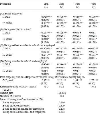
For most of the paper, our sample consists of unmarried men aged 17–24 who have no children, are not members of the Armed Forces, are not permanently un-able to work, live in one of the ten Canadian provinces, and are either employed as paid workers or not employed.8,9 When selecting individuals who are employed as paid workers, we restrict our attention to individuals who worked no more than 85 hours per week and who earned at least $5.00 per hour in 2002 dollars.10 Individu-als aged 17–20 with a university degree and those aged 17–18 with trades certifi -cates or diplomas represent a negligible fraction of unmarried men aged 17–24 and thus are excluded from the analyses. Of all young men in the resulting sample, 58.6 percent were employed in 2001, 51.9 percent were enrolled in school, 11.8 percent were neither in school nor employed, and 22.3 percent combined school and work (Table 1).
In most of the paper, we consider fi ve binary outcomes: (1) being employed; (2) be-ing enrolled in school; (3) bebe-ing enrolled in university full time; (4) bebe-ing neither en-rolled in school nor employed; and (5) being both enen-rolled in school and employed.11 Our empirical strategy relates the outcome of individual i in age group a with edu-cation level e, living in region r in year t, Yiaert, to his/her log after- tax hourly wages, lnWiaert, a vector of individual- level control variables, Xiaert,and a vector of age/educa-tion/region- specifi c controls, Zaert, through the following equation:
7. This sample selection scheme implies that some individuals may be observed twice in a given year (or two different years) within a given age*education*region combination. Because the regression analyses used in the study are based on standard errors clustered at the age*education*region level, these analyses allow arbi-trary serial correlation that could result, among other factors, from multiple observations originating from the same individuals. Another concern is that as they get older or increase their education level, some individuals may contribute one observation to a given age*education*region cluster and another observation to a differ-ent cluster. This might induce cross- cluster correlation. Removing these individuals from the basic sample reduces sample sizes by about 3 percent and does not alter the main findings of this study.
8. Self- employed individuals are excluded. Self- employment rates of unmarried men aged 17 to 24 averaged about 2 percent during the 2001–2008 period and displayed no trend. As a result, excluding self- employed individuals is unlikely to bias our results.
9. 2SLS analyses are limited to young men because the instrumental variable used in this study is not strongly correlated with young women’s hourly wages, thereby precluding the use of an IV estimator for young women. This finding is expected given that relatively few young women are employed in the oil in-dustry.
10. Since province- specific minimum wages ranged from $5.63 to $8.00 (in 2002 dollars) between 2001 and 2008, the $5.00 wage restriction rules out unusually low wages.
Table 1
Real Wages and Young Men’s Outcomes
Percentile 15th
(1)
25th (2)
35th (3)
45th (4)
(A) Being employed
I. OLS 0.939*** 0.706*** 0.460*** 0.190***
(0.039) (0.031) (0.027) (0.021)
II. 2SLS 0.347*** 0.380*** 0.430*** 0.470***
(0.089) (0.103) (0.120) (0.139) (B) Being enrolled in school
I. OLS –0.197*** –0.125*** –0.048† 0.031
(0.023) (0.026) (0.028) (0.028)
II. 2SLS –0.260* –0.284* –0.322* –0.351*
(0.108) (0.122) (0.141) (0.158) (C) Being neither enrolled in school nor employed
I. OLS –0.309*** –0.237*** –0.156*** –0.062**
(0.018) (0.014) (0.010) (0.007)
II. 2SLS –0.141*** –0.154*** –0.175*** –0.191**
(0.042) (0.047) (0.054) (0.061) (D) Being enrolled in school and employed
I. OLS 0.434*** 0.344*** 0.256*** 0.159***
(0.054) (0.046) (0.039) (0.030)
II. 2SLS –0.054 –0.059 –0.067 –0.073
(0.069) (0.076) (0.087) (0.095) First-stage regressions (Dependent variable is log after-tax real hourly wages)
OIL_aert 2.37*** 2.16*** 1.91*** 1.75***
(0.28) (0.30) (0.29) (0.30)
Kleibergen-Paap Wald F statistic (2SLS)
73.0 52.8 42.2 34.8
Sample size 170,632
Number of clusters 164
Mean of young men’s outcomes in 2001
Being employed 0.586
Being enrolled in school 0.519
Being neither in school nor employed 0.118 Being enrolled in school and employed 0.223
Source: Authors’ calculations from Labour Force Survey.
(1) Yiaert =aer+t +1* lnWiaert+ Xiaert*2+ Zaert*3+iaert
t =2001, …2008
where aer and t capture age- education- region (group) fi xed effects and year effects, respectively, and where iaert is an error term.12,13 The vector X
iaert consists of binary
indicators for individuals: (1) living in a census metropolitan area (CMA) or a census agglomeration (CA); (2) belonging to a household that rents its dwelling; and (3) sam-pled in February, March, or October (September being the reference month). The vec-tor Zaert controls for labor market conditions and includes the unemployment rate and
the rate of involuntary part- time employment of young men in age group a, with edu-cation level e, living in region r in year t.
Since wages are unobserved for nonemployed men, we impute wage offers for these individuals using various percentiles, PCTLp
aert, of the log after- tax wage distribution
of employed men in age group a, with education level e, living in region r in year t. The resulting wage variable, lnWp
iaert, combines these imputed values for
nonpartici-pants and the observed wages for particinonpartici-pants, thereby yielding the following equation:
(2) Yiaert =aer+t +1* lnW
p
iaert+ Xiaert*2+ Zaert*3+iaert t =2001, … 2008.
To ensure that results are robust to the choice of imputed values, we construct vari-ous estimates of lnWp
iaert based on the 15th, 25th, 35th, or 45th percentile of the cell-
specifi c wage distributions defi ned above. Because lnWp
iaert and iaert may be correlated due to unobserved heterogeneity or
measurement error in after- tax hourly wages, we instrument lnWp
iaert with OILaert≡(OIL_PRICEt -1 / 100)* OIL_SHAREaer_9700. This instrumental variable is the
product of last year’s oil prices and the share of employed young men (in age group a
and education level e living in region r) working in the oil industry between 1997 and 2000 (OIL_SHAREaer_9700).14 The rationale for this instrument is simple: For a given
increase in oil prices, labor demand, and thus wages, should grow faster among groups of young men who were heavily involved in the oil industry prior to the 2000s than
12. After- tax hourly wages are computed as follows. First, weekly earnings of paid workers (measured in current dollars) are multiplied by 52 weeks and converted into hypothetical annual earnings. Second, a Canadian tax calculator provided by Milligan (2012) is used to calculate after- tax hourly wages in current dollars. Third, using province- specific Consumer Price Indexes (All items), real after- tax hourly wages are constructed.
13. Four age groups (17–18, 19–20, 21–22, 23–24), seven education levels (Grade 10 or lower; Grade 11, 12, or 13 with no high school diploma; high school diploma; trades certificate or diploma; some postsecond-ary education; college, CEGEP, and university certificate below bachelor’s degree; and bachelor’s degree or above), and eight regions (one region encompassing New Brunswick, Nova Scotia, and Prince Edward Island, and one region for each of the remaining provinces) are considered each year.
among other groups.15 Because increases in world oil prices may trigger increases in youth wages with a certain lag, the one- year lagged value of oil prices is used when constructing OILaert.
The instrument above is defi ned for 200 groups of workers tracked over eight years, thereby potentially yielding variation based on up to 1,600 age*education*region*year observations.16,17 To ensure that imputed wage offers are based on reasonable samples of employed young men, we restrict our analyses to groups of individuals for whom wages are imputed on the basis of at least 20 (microdata observations of ) employed individuals. These restrictions yield a basic sample of 170,632 observations, from which 1,128 age*education*region*year grouped observations on OILaert and Zaert can be obtained. These 1,128 grouped observations are related to 164 (age/education/ region- specifi c) groups of young men and are based on microdata samples that contain 151.3 observations, on average.
While the instrumental variable estimation strategy described above takes advantage of cross- group variation in wage growth induced by a specifi c shock—increases in world oil prices—an alternative is to use a grouping estimator that exploits all cross- group variation in wage growth. If changes in real wages across groups (defi ned by age, education, and region) are driven by shifts in labor demand unrelated to Canadian young men’s school enrollment and labor supply decisions18, then a grouping estima-tor can be used to estimate the following model19:
(3) Yaert =aer+t +1* lnWpaert+ Xaert*2+ Zaert*3+aert t =2001, … 2008
where the dependent variable and the regressors have been redefi ned at the group level. We estimate Equation 3 separately for the aforementioned sample of young men and for a comparable sample of young women, thereby comparing youth responses to wages across gender.20
To assess whether the grouping estimator associated with Equation 3 is subject to attenuation bias due to small sample sizes within some cells, we use two strategies. First, we replace our basic group defi nition by an alternative defi nition in which indi-viduals are classifi ed into two age groups (17–20, 21–24) rather than four age groups
15. An alternative scenario is that, as energy prices rise, the use of capital decreases, and the demand for unskilled labor—relative to skilled labor—increases, thereby lowering the skill wage premium within prov-inces (Polgreen and Silos 2009), a pattern observed in the data.
16. The 200 groups result from the interaction of eight regions and 25 age- education cells. These 25 age- education cells in turn are obtained by removing three age- education combinations (individuals aged 17–18 with trades certificates or diplomas; individuals aged 17–18 with a bachelor’s degree or above; and individu-als aged 19–20 with a bachelor’s degree or above) from a set of seven education levels interacted with four age groups.
17. Since oil prices likely increased wages directly or indirectly (through spillover effects) only for a subset of young men, our 2SLS estimates should be interpreted as local average treatment effects rather than overall average treatment effects.
18. Differential changes in the worldwide supply of workers across skill groups, the appreciation of the Canadian dollar on the foreign exchange market, and the drop in real interest rates during the 2000s may have generated differential changes in domestic labor demand across industries and, thus, in youth labor demand across groups.
19. Several studies (Blundell, Duncan, and Meghir 1998; Devereux 2004, 2007a, 2007b; Blau and Kahn 2007) use grouping estimators to estimate labor supply models.
(17–18, 19–20, 21–22, 23–24), thereby increasing average sample size per cell.21 For both defi nitions, seven education levels and eight regions are considered. In both cases, we estimate Equation 3 using the effi cient Wald estimator (EWALD), which we implement using weighted least squares, where the weights represent population estimates in a given cell.22 In addition, we estimate Equation 3 using the unbiased error- in- variables estimator (UEVE) developed by Devereux (2007a; 2007b).
As they consider whether to stay in school, individuals may compare their current wage offers to those they are likely to receive after completing additional schooling (Becker 1964; Black, McKinnish, and Sanders 2005). If so, Equations 2 and 3 should be re- estimated using a variable that captures relative wages rather than real wages. For this reason, alternative versions of Equations 2 and 3 are also considered. In the alternative versions of Equation 2, log real wages (lnWp
iaert) are replaced by
lnW
p*
iaert ≡ ln[W p
iaert / W25-29_RF_rt,t -1], where W25-29_RF_rt, t -1 denotes the average after-
tax real hourly wages received in region r in years t and t- 1 by employed young men aged 25–29 belonging to a given reference group.23 In the alternative versions of Equation 3, lnWp
aert is replaced by lnW p*
aert ≡ ln[Wpaert / W25-29_RF_rt, t -1].
Apart from variability in the temporal patterns observed across age groups and edu-cation levels, the identifi cation strategy relies on cross- provincial variation in the evo-lution of young men’s outcomes and wages. Because the analysis is based on a time series of cross- sections, the fi ndings might be affected by selective interprovincial migration. While the LFS contains no information that distinguishes stayers from mi-grants, Statistics Canada’s Longitudinal Administrative Databank (LAD) can be used to deal with selective interprovincial migration. We use LAD to assess whether the oil- producing provinces lost (gained) ground relative to the other provinces, in terms of university enrollment (employment) rates, to a similar extent in a basic sample— which includes migrants and stayers—versus a sample that consists exclusively of stayers. As will be shown below, these comparisons reveal that cross- provincial move-ments in university enrollment and employment are not driven simply by selective interprovincial migration.
A. Instrument Validity
There are several threats to the validity of our instrumental variable. Equation 2 as-sumes that increases in oil prices affect young men’s school enrollment only through increased wages. Yet positive oil price shocks may affect enrollment through other channels as well. A priori, they can improve young men’s employment opportunities andboost the asset income or employment income of their parents. By increasing revenues of oil- producing provinces and aggregate demand for labor, increases in oil prices might induce provincial governments to increase spending on education, lower
21. As will be shown below, using the alternative group definition raises average sample size per cell from 151.3 to 243.2 observations for young men and from 148.1 to 234.5 observations for young women. 22. Standard errors for Equations 2 and 3 are clustered at the age- education- region level, thereby allowing for serial correlation of an unspecified nature within age- education- region cells. In most of the paper, Equa-tion 2 is estimated using LFS sampling weights.
university tuition fees, modify social assistance parameters, and/or raise minimum wages. All of these factors can potentially affect young men’s school enrollment and university attendance.
We address these issues as follows. First, we include controls for young men’s un-employment rates and rate of involuntary part- time un-employment in Equation 2. Doing so rules out the possibility that young men reduce their school enrollment simply be-cause there are more jobs available, rather than bebe-cause of higher wage offers.24 Sec-ond, we note that increases in parental income triggered by rising oil prices are, if anything, likely to foster young men’s school enrollment by (potentially) increasing university attendance. If so, they will bias upward our estimates of 1, thereby yielding conservative estimates of the degree to which high wages reduce school enrollment and university attendance. A similar argument applies to the omission of government spending on education in Equation 2. Third, we use augmented versions of Equations 2 and 3 that control for province- specifi c: (a) log average real tuition fees associated with a bachelor’s degree; (b) levels of real income from social assistance potentially available to nonemployed single individuals; and (c) log real minimum wages.25 As a result, our estimates of 1 are not contaminated by these factors.26,27 However, in-creases in parental income and in government spending on education will lead to a reduction in the proportion of young men neither enrolled in school nor employed if they lead to a rise in school enrollment among young men who were initially not em-ployed. The same factors will increase the proportion of young men both enrolled and employed if they raise school enrollment among employed young men. If so, estimates of 1 will capture the joint infl uence of increased wages, increased parental income, and increased government spending on the proportion of young men: (a) neither en-rolled in school nor employed, (b) both enen-rolled and employed. While this possibility cannot be ruled out, we reduce concerns about it by estimating alternative versions of
24. Young men’s rates of unemployment and of involuntary part- time work are defined as ratios of the number of individuals unemployed or involuntarily employed part time to the population of young men. Both variables are endogenous with respect to school enrollment. However, estimates of the impact of wages will remain consistent as long as the (oil price) instrument used in this study is uncorrelated with the error term after conditioning on observables (including unemployment and involuntary part- time work) (Stock and Watson 2011). Contrary to the estimated wage impact, the parameter estimates for youth unemployment and involuntary part- time employment will not have a causal interpretation, however.
25. Province- specific/year- specific social assistance incomes are obtained from the report titled Welfare In-comes 2009, published by the National Council of Welfare (National Council of Welfare 2010). The calcula-tions from the National Council of Welfare assume that: (a) recipients first received welfare benefits on Janu-ary 1; (b) this is the very first time they have ever received welfare benefits; (c) recipients reside in the largest city or town in their province or territory; (d) there are no penalties for being new to the area; (e) recipients live in private rental accommodation and do not share; (f ) recipients receive the highest level of shelter as-sistance for tenants, whereby all utility costs are included; (g) there are no costs for moving; and h) there are no costs for repairing the rental accommodation.
26. Because these three variables are defined at the province or region level (rather than at the age*education*region level), their inclusion raises issues of multiple levels of clustering and of relatively few clusters at the higher level (region or province) when standard errors are computed. To ensure that the main
findings of this study are not affected by such issues, all models have been re- estimated without controls for tuition fees, potential income from social assistance, and minimum wages. Omitting these factors does not alter the main findings of the study.
Equation 3 that are augmented with province- specifi c linear trends.28 If parental in-come and government resources spent on education increased faster in oil- producing provinces than in other provinces and are the main factors that reduced the proportion of young men neither enrolled in school nor employed, estimates of 1 should drop substantially when moving from Equation 3 to alternative versions that include these trends. We fi nd no such evidence: Most of the estimated impact of real wages on young men’s likelihood of being neither in school nor employed generally remains in the aggregate when we use these alternative versions of Equation 3. Whether we aug-ment Equation 3 with province- specifi c trends or not, we generally detect no statisti-cally signifi cant impact of real wages on young men’s likelihood of being both en-rolled in school and employed at the aggregate level. Furthermore, our 2SLS point estimates of 1 (in models of young men’s propensity to combine school and work) are negative in the aggregate, even though they are potentially biased upward. Hence, our main results regarding young men’s probability of being neither enrolled in school nor employed (or being both enrolled and employed) do not appear to be driven by the omission of parental income or government spending on education.
B. Instrument Relevance
Tables 1 to 3 show that the instrument selected is strongly correlated with log after- tax real wages. For all models and samples considered in these tables, the Kleibergen- Paap Wald F- statistic for OILaert ranges from 10.0 to 73.0. As expected, increased oil prices are positively correlated with real wages, with coeffi cients for OILaert generally close to 2.0. This suggests that a doubling of oil prices from their 2002 level would increase by roughly ten points the (log) after- tax real wages of young men for whom the prob-ability of working in the oil industry was equal to 5 percent during the 1997–2000 period.29
C. Identifi cation
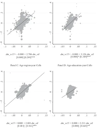
In Figure 1, we group the data on log after- tax real wages and our instrumental vari-able in several ways to assess which dimensions—age, education, region—provide identifi cation of wage impacts. Figures 1a, 1b, and 1c show that movements in oil prices are strongly positively correlated with changes in young men’s real wages when the data is grouped by age*education*region, education*region or age*region. Figure 1d shows that this correlation is not as strong and that movements in our in-strumental variable are more limited when the data is grouped by age*education. This
28. The same procedure cannot be used for Equation 2 since our instrumental variable becomes a weak in-strument when province- specific trends are added to this equation. This is expected since the identification strategy used relies partly on cross- provincial variation in wage growth and youth outcomes.
Table 2
Real Wages and Outcomes of Young Men with a High School Diploma or More Education
Percentile 15th (C) Being neither enrolled in school nor employed
I. OLS –0.278*** –0.214*** –0.139*** –0.056***
(0.018) (0.015) (0.011) (0.007)
II. 2SLS –0.091* –0.095* –0.106* –0.114*
(0.039) (0.031) (0.046) (0.049) (D) Being enrolled in school and employed
I. OLS 0.374*** 0.301*** 0.223*** 0.140***
(0.051) (0.046) (0.038) (0.031)
II. 2SLS –0.146† –0.154† –0.171† –0.183†
(0.076) (0.081) (0.091) (0.099) First-stage regressions (Dependent variable is log after-tax real hourly wages)
OIL_aert 2.50*** 2.38*** 2.14*** 2.00***
(0.35) (0.39) (0.38) (0.39)
Kleibergen-Paap Wald F statistic (2SLS)
50.3 37.2 31.0 26.1
Sample size 119,750
Number of clusters 116
Mean of young men’s outcomes in 2001
Being employed 0.625
Being enrolled in school 0.472
Being neither in school nor employed 0.110 Being enrolled in school and employed 0.207
Source: Authors’ calculations from Labour Force Survey.
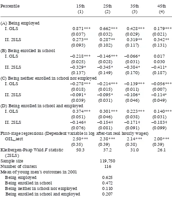
Notes: The sample consists of unmarried men aged 17–24 with no children and who have a high school diploma, a trades certifi cate or diploma, or more education. The numbers show the estimated impact of log after- tax real wages on the probability of being employed, being enrolled in school, being neither enrolled in school nor employed, and being both enrolled in school and employed. Separate regressions are run based on various percentiles used for im-puting the wages of nonemployed men. All regressions include group fi xed effects, year effects, month indicators, a renter indicator, a CMA / CA indicator, the unemployment rate, and the rate of involuntary part- time employment defi ned at the age*education*region level, as well as province- specifi c log real minimum wages, log average real tuition fees for a bachelor’s degree, and levels of Social Assistance income potentially available to single individu-als. Standard errors clustered at the age*education*region level are between parentheses.
Table 3
Real Wages and Outcomes of Young Men with No High School Diploma
Percentile 15th (C) Being neither enrolled in school nor employed
I. OLS –0.454*** –0.353*** –0.238*** –0.094***
(0.054) (0.044) (0.032) (0.022)
II. 2SLS –0.226* –0.275* –0.321† –0.371†
(0.112) (0.139) (0.172) (0.204) (D) Being enrolled in school and employed
I. OLS 0.723*** 0.564*** 0.429*** 0.257**
(0.156) (0.125) (0.108) (0.076)
II. 2SLS 0.246† 0.299† 0.350† 0.404†
(0.145) (0.168) (0.185) (0.221) First-stage regressions (Dependent variable is log after-tax real hourly wages)
OIL_aert 2.01*** 1.66*** 1.42*** 1.23***
(0.45) (0.42) (0.43) (0.39)
Kleibergen-Paap Wald F statistic (2SLS)
20.5 15.6 10.7 10.0
Sample size 50,882
Number of clusters 48
Mean of young men’s outcomes in 2001
Being employed 0.497
Being enrolled in school 0.624
Being neither in school nor employed 0.136 Being enrolled in school and employed 0.258
Source: Authors’ calculations from Labour Force Survey.
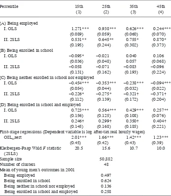
Notes: The sample consists of unmarried men aged 17–24 with no children and with no high school diploma. The numbers show the estimated impact of log after- tax real wages on the probability of being employed, being enrolled in school, being neither enrolled in school nor employed, and being both enrolled in school and employed. Separate regressions are run based on various percentiles used for imputing the wages of nonemployed men. All regressions include group fi xed effects, year effects, month indicators, a renter indicator, a CMA / CA indicator, the unemploy-ment rate, and the rate of involuntary part- time employunemploy-ment defi ned at the age*education*region level, as well as province- specifi c log real minimum wages, log average real tuition fees for a bachelor’s degree, and levels of Social Assistance income potentially available to single individuals. Standard errors clustered at the age*education*region level are between parentheses.
Panel A: Age-education-region-year Cells
Panel C: Age-region-year Cells
Panel B: Education-region-year Cells
Panel D: Age-education-year Cells
–.
4
–.
2
.2
0
.4
–.1 –.05 0 .05 .1 .15
–.
4
–.
2
.2
0.
4
–.1 –.05 0 .05 .1 .15
–.
4
–.
2
.2
0.
4
–.1 –.05 0 .05 .1 .15
–.
4
–.
2
.2
0.
4
–.1 –.05 0 .05 .1 .15
dm_w15 = – 0.000 + 2.706 dm_oil dm_w15 = – 0.000 + 3.126 dm_oil
[0.000] [0.289]*** [0.000]* [0.349]***
dm_w15 = 0.000 + 2.801 dm_oil dm_w15 = 0.000 + 2.211 dm_oil
[0.001] [0.561]*** [0.000] [0.645]**
Figure 1
Log After- tax Real Wages and Oil Prices
Notes: Deviations over time of log after- tax real wages from group- specifi c means on the Y- axis are plotted against oil prices (demeaned) on the X- axis. Log after- tax real wages from wage imputations (for nonemployed young men) based on the 15th percentile. A linear fi t is plotted and the resulting equation is shown under each panel. Standard errors from these weighted regressions are clustered at the group level and are between brackets.
suggests that most of the identifi cation comes from cross- regional variation in young men’s wage growth and in changes in our instrumental variable.30
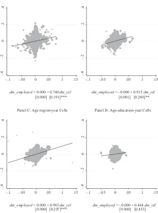
Likewise, Figures 2a– 2d indicate that movements in young men’s employment rates and in our instrumental variable are more strongly correlated when the data is grouped at least by region (Figures 2a–2c) than when it is not (Figure 2d). Together, Figures 1 and 2 suggest that identifi cation of the impact of wages on young men’s employment originates mainly from cross- regional variation in young men’s employment move-ments, wage growth, and exposure to rising oil prices. Graphical analysis of other outcomes also suggests a predominant identifi cation role for cross- regional variation in young men’s wage growth and in changes in our instrumental variable.
IV. Results
Table 1 presents OLS and 2SLS results from Equation 2 estimated on the sample of young men using our basic group defi nition, in which group fi xed effects aer are defi ned by the interaction of four age categories, seven education levels, and eight regions. Four outcomes are considered: being employed, being enrolled in school, being neither enrolled in school nor employed, and being both enrolled in school and employed. For each outcome, separate regressions are run based on various percentiles used for imputing wages of nonemployed men.
For all estimators and percentiles considered, increased real wages unambiguously raise young men’s employment rate and reduce their probability of being neither en-rolled in school nor employed. The 2SLS estimator suggests that a ten- point increase in log after- tax real wages (0.10) raises young men’s employment rate by 3.5 to 4.7 percentage points.31 Since roughly 59 percent of young men were employed in 2001, these numbers imply wage elasticities of labor market participation that range from 0.59 (0.35/0.59) to 0.80 (0.47/0.59).32 In addition, 2SLS parameter estimates show that a ten- point increase in log after- tax real wages lowers young men’s likelihood of be-ing neither in school nor employed by 1.4 to 1.9 percentage point and reduces young men’s school enrollment rate by 2.6 to 3.5 percentage points, from a baseline (2001) school enrollment rate of 52 percent. Contrary to OLS results, 2SLS estimates do not support the hypothesis that increased wages induce male students to start combining
30. Cross- regional variation in changes in our instrumental variable is driven by cross- regional variation in young men’s employment shares in the oil industry during the 1997–2000 period.
31. In contrast, minimum wage parameter estimates indicate that a ten- point increase in log real minimum wages is associated with a drop in employment rates of roughly one percentage point (Appendix Table A1). Results not shown indicate that income from social assistance potentially available to nonemployed single males is uncorrelated with employment rates.
32. Comparing these numbers with those of Gustman and Steinmeier (1981) is difficult since they report no wage parameter estimates or wage elasticities. Using SIPP US data from May 1983 to April 1986, Kimmel and Kniesner (1998) find an employment elasticity of 0.65 for (a sample that includes both young and older) single men. Using more recent data on samples of individuals aged 18–59, Bargain, Orsini, and Peichl (2012) compute labor supply elasticities for 17 European countries and the United States. For single men, they find that wage elasticities at the extensive margin range from 0.04 to 0.62 with a cross- country mean of 0.23. Because we focus on young single men (aged 17–24 rather than 18–59), we expect to find—and we do
Panel A: Age-education-region-year Cells
Panel C: Age-region-year Cells
Panel B: Education-region-year Cells
Panel D: Age-education-year Cells dm_employed = 0.000 + 0.740 dm_oil dm_employed = –0.000 + 0.915 dm_oil
[0.000] [0.191]*** [0.001] [0.280]**
dm_employed= 0.000 + 0.983 dm_oil dm_employed = –0.000 + 0.444 dm_oil
[0.000] [0.207]*** [0.000] [0.453]
–.
4
–.
2
.2
0
.4
–.1 –.05 0 .05 .1 .15
–.
4
–.
2
.2
0.
4
–.1 –.05 0 .05 .1 .15
–.
4
–.
2
.2
0.
4
–.1 –.05 0 .05 .1 .15
–.
4
–.
2
.2
0.
4
–.1 –.05 0 .05 .1 .15
Figure 2
Young Men’s Employment Rates and Oil Prices
Notes: Deviations over time of young men’s employment rates from group- specifi c means on the Y- axis are plotted against oil prices (demeaned) on the X- axis. A linear fi t is plotted and the resulting equation is shown under each panel. Standard errors from these weighted regressions are clustered at the group level and are between brackets.
school and work: Estimates of 1, which are positive with OLS, become negative and imprecisely measured under 2SLS.
In sum, our main fi nding is that following improved wage offers, young men gen-erally increase their labor market participation though two channels: (a) a reduction in school enrollment and; (b) the (re- )entry into the labor market of some individu-als who were neither in school nor employed. Estimates from 2SLS provide no evi-dence—at least in the aggregate—that young men start combining school and work in greater numbers in response to increased wages.
These qualitative patterns hold when we restrict our attention to young men with a high school diploma, a trades certifi cate or diploma, or more education (henceforth, young men with a high school diploma or more education) (Table 2). For this subsam-ple, the 2SLS estimator indicates that a ten- point increase in log after- tax real wages raises labor market participation by between 2.7 and 3.4 percentage points, reduces school enrollment by between 3.3 and 4.1 percentage points, and lowers the likelihood of being neither in school nor employed by between 0.9 and 1.1 percentage point.
A different story emerges for young men with no high school diploma. For this subsample, there is virtually no evidence that increased wages lead to a drop in school enrollment. Only OLS parameter estimates based on the 15th percentile are negative and statistically signifi cant at conventional levels in school enrollment equations (Table 3). In response to improved wage offers, less- educated young men appear to increase their labor market participation by making transitions from be-ing neither in school nor employed into employment and by combinbe-ing school and work in greater numbers. Parameter estimates from 2SLS indicate that a ten- point increase in log after- tax real wages boosts labor market participation by between 5.3 and 8.7 percentage points, from a baseline employment rate of about 50 percent. These numbers imply a substantial wage elasticity of labor market participation for less- educated young men that varies between 1.07 and 1.75.33,34 A ten- point increase in log after- tax real wages also lowers the likelihood of being neither in school nor employed by between 2.3 and 3.7 percentage while increasing the proportion of individuals who combine school and work by between 2.5 and 4.0 percentage points.
V. Robustness Checks
A. Estimator Choice, Model Specifi cation, and Weighting Scheme
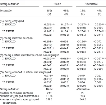
Our main fi nding is robust to the use of alternative: (a) estimators, (b) functional forms, and (c) weighting schemes. First, most of the patterns found in Table 1 under 2SLS hold when we use grouping estimators (EWALD and UEVE) and two group defi nitions: (a) a basic defi nition, in which group fi xed effects fully interact four age
33. The large participation wage elasticity we find for young men with no high school diploma is consistent with the finding of Bargain, Orsini, and Peichl (2012) that wage elasticities for single men are higher at lower- income quintiles than at other quintiles.
Table 4
Real Wages and Young Men’s Outcomes – Grouping Estimators
Group defi nition Basic Alternative
Percentile 15th
(1)
45th (2)
15th (3)
45th (4)
(A) Being employed
I. EWALD 0.256*** 0.137*** 0.267*** 0.180***
(0.034) (0.037) (0.040) (0.040)
II. UEVE 0.165*** 0.124*** 0.204*** 0.174***
(0.028) (0.031) (0.031) (0.034) (B) Being enrolled in school
I. EWALD –0.101* –0.036 –0.136** –0.072
(0.042) (0.049) (0.048) (0.055)
II. UEVE –0.085** –0.045 –0.127** –0.082*
(0.031) (0.033) (0.035) (0.037) (C) Being neither enrolled in school nor employed
I. EWALD –0.082*** –0.063** –0.082*** –0.087***
(0.021) (0.022) (0.023) (0.021)
II. UEVE –0.042* –0.058** –0.053** –0.084***
(0.018) (0.019) (0.018) (0.019) (D) Being enrolled in school and employed
I. EWALD 0.073† 0.038 0.049 0.021
(0.040) (0.041) (0.043) (0.046)
II. UEVE 0.037 0.022 0.024 0.008
(0.026) (0.027) (0.029) (0.030)
Group defi nition Basic Alternative
Number of clusters (groups) 164 97
Number of grouped observations 1,128 729
Average sample size per grouped observation
151.3 243.2
Source: Authors’ calculations from Labour Force Survey.
Notes: The sample consists of unmarried men aged 17–24 with no children. The numbers show the estimated impact of log after- tax real wages on the probability of being employed, being enrolled in school, being neither enrolled in school nor employed, and being both enrolled in school and employed. Separate regressions are run based on various percentiles used for imputing the wages of nonemployed men. All regressions include group fi xed effects, year effects, month indicators, a renter indicator, a CMA / CA indicator, the unemployment rate, and the rate of involuntary part- time employment defi ned at the age*education*region level, as well as province- specifi c log real minimum wages, log average real tuition fees for a bachelor’s degree, and levels of Social Assistance income potentially available to single individuals. Standard errors clustered at the age*education*region level are between parentheses for EWALD.
categories, seven education levels, and eight regions; and (b) an alternative defi nition, which interacts two age groups with the (seven) education and (eight) region catego-ries (Table 4). While estimates from grouping estimators are generally smaller in abso-lute value than those from 2SLS, they confi rm that increased real wages are associated with rising employment rates and a reduced likelihood of young men being neither in school nor employed.35 UEVE estimates also confi rm that increased real wages reduce school enrollment: Of the eight wage parameter estimates (four of which are shown in Table 4) associated with the two group defi nitions and the four percentiles considered, six are statistically signifi cant at the 5 percent level.
Second, our main fi nding is robust to functional form. As Appendix Table A2 shows, moving from a level- log wage model to a log- log wage model when using EWALD (and our basic group defi nition) yields fairly similar wage elasticities of employment and the likelihood of being neither in school nor employed, both for all young men and for young men with a high school diploma or more education. For these two samples, wage elasticities of school enrollment increase in absolute value when moving to log- log specifi cations, thereby strengthening our fi nding that reductions in school enrollment are a second channel through which relatively more- educated young men increase their labor market participation.36
Third, considering all young men or those with a high school diploma or more education, both weighted and unweighted 2SLS estimates confi rm that the growth in young men’s labor market participation that follows rising wages comes from a drop in school enrollment and the (re- )entry into the labor market of some who were neither in school nor employed rather than an increase in the proportion combining school and work (Appendix Table A3). Unweighted 2SLS estimates also confi rm that young men with no high school diploma do not appear to reduce school enrollment following improved wage offers. For this subsample, unweighted wage parameter estimates for various outcomes are generally insignifi cant at conventional levels.
B. Source of Decline in School Enrollment
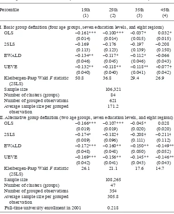
In Table 5, we investigate the source of the reduction in school enrollment found in Tables 1 and 2. To do so, we show the estimated impact of real wages on full- time uni-versity enrollment for potential male uniuni-versity enrollees.37 The fi rst and second pan-els of Table 5 present results from all estimators (OLS, 2SLS, EWALD, and UEVE) using the basic group defi nition and the alternative group defi nition, respectively.
35. In seven cases out of eight (defined by four percentiles and the two group definitions), most of the esti-mated EWALD impact of real wages on young men’s likelihood of being neither in school nor employed remains when adding province- specific trends to Equation 3. This suggests that the estimates shown in Table 4 are not driven solely by the omission of time- varying factors such as parental income and government spending on education.
36. Wage elasticities of school enrollment also increase, in absolute value, for young men with no high school diploma. However, whether we use real wages or relative wages, these elasticities are not statistically significant at conventional levels for most percentiles considered.
Table 5
Real Wages and Full- Time University Enrollment – Potential Male University Enrollees
Percentile 15th
I. Basic group defi nition (four age groups, seven education levels, and eight regions)
OLS –0.161*** –0.100*** –0.037* 0.032* Kleibergen-Paap Wald F statistic
(2SLS)
50.8 36.8 29.4 26.9
Sample size 106,321
Number of clusters (groups) 84
Number of grouped observations 621 Average sample size per grouped
observation
171.2
II. Alternative group defi nition (two age groups, seven education levels, and eight regions)
OLS –0.166*** –0.107*** –0.045* 0.028 Kleibergen-Paap Wald F statistic
(2SLS)
26.1 21.1 17.6 14.7
Sample size 108,265
Number of clusters (groups) 47
Number of grouped observations 354 Average sample size per grouped
observation
305.8
Full-time university enrollment in 2001 0.218
Source: Authors’ calculations from Labour Force Survey.
Notes: The sample consists of unmarried men aged 17–24 with no children and who have a high school diploma, some postsecondary education, a college diploma, a CEGEP diploma, or a university certifi cate below bachelor’s degree. The numbers show the estimated impact of log after- tax real wages on the probability of attending uni-versity on a full- time basis. All models include group fi xed effects, year effects, and all other regressors used in Tables 1–3. Standard errors clustered at the age*education*region level are between parentheses for OLS, 2SLS, and EWALD.
The fi rst observation is that under the basic group defi nition, 2SLS estimates indi-cate that a ten- point increase in log after- tax real wages reduces full- time university enrollment by roughly two percentage points, from a baseline enrollment rate of 22 percent. However, the wage parameters are estimated imprecisely. Using the alterna-tive group defi nition yields similar but more precisely estimated 2SLS parameters that are statistically signifi cant at the 6 percent level.38 Using grouping estimators with the alternative group defi nition—under which sample size per cell averages 305.8 obser-vations—yields parameters that are estimated even more precisely. These parameters suggest that a ten- point increase in log after- tax real wages reduces full- time uni-versity enrollment by about 1.5 percentage point. In addition, re- estimating EWALD and UEVE with log after- tax relative wages (under the alternative group defi nition) indicates that a ten- point increase in log relative wages lowers full- time university enrollment by between 1.0 and 1.3 percentage point.39 Together, these results confi rm that declines in full- time university enrollment underlie part of the drop in school enrollment shown in Tables 1 and 2.40
Could this drop in school enrollment also come from less- educated young men leav-ing school in response to increased wages? While 2SLS results detect no statistically signifi cant reduction in school enrollment for young men with no high school diploma, these results are potentially biased upward due to the omission of parental income and government spending on education. Since our instrumental variable is weakly cor-related with wages when province- specifi c trends are added to Equation 2, we cannot assess how the 2SLS wage parameters of the school enrollment equation change when adding these trends. For this reason, we pursue a different strategy. To allow for the possibility that parental income and government spending on education might have risen faster in oil- producing provinces than in other provinces, we estimate an alterna-tive version of Equation 3 that includes province- specifi c trends. We then compare the resulting estimates to those obtained from Equation 3. We do so using our basic group defi nition. Whether we use EWALD or UEVE, real wages or relative wages, and include province- specifi c trends or not in Equation 3, we fail to detect a negative and statistically signifi cant school enrollment response to increased wages for young men with no high school diploma (results available in Table 3.1 in the online appendix). Combined with the possibility that selective interprovincial migration might lead to a spurious drop in school enrollment among this group in oil- producing provinces41, this fi nding provides additional evidence that the reduction in school enrollment found in the aggregate does not originate from young men with no high school diploma.
38. Under this alternative group definition, we also get fairly similar 2SLS estimates that are statistically significant at the 8 percent level when we impute wages of nonemployed male potential university enrollees using the 55th, 65th, 75th, or 85th percentile of cell- specific wage distributions. Results are available on Table 5.1 in the web appendix that can be found at http://jhr.uwpress.org/.
39. All underlying parameters are statistically significant at the 5 percent level. Results are available on Table 5.2 in the web appendix.
40. In contrast, regression analyses of full- time enrollment in community colleges, junior colleges, or CEGEPs yield little evidence that increased (real or relative) wages reduce full- time attendance in these postsecondary institutions.
C. Selective Migration
The results presented so far take no account of selective interprovincial migration. If young male migrants predominantly consist of individuals who have already com-pleted their schooling, are already employed in their province of origin, and have moved to oil- producing provinces after accepting a better- paid job in these provinces, both university enrollment rates and the likelihood of young men being neither en-rolled in school nor employed will fall in the oil- producing provinces relative to the other provinces, even if wages have no causal impact on these outcomes. Thus, selec-tive migration may lead us to overstate the impact of wages on university enrollment, young men’s employment, and the likelihood of young men being neither enrolled in school nor employed.
The LAD, a large Canadian administrative data set, is used to address this issue. Since 1999, the LAD has contained information on educational deductions for part- time students and full- time students as well as information on tuition fees paid to postsecondary educational institutions. As a result, the LAD allows the estimation of full- time university enrollment rates for the observation period considered in this study.42 Because it contains a 20 percent random sample of all Canadian tax fi lers, the LAD yields very large sample sizes. This allows us to estimate separate models for: (a) a basic sample that includes both interprovincial migrants and stayers; and (b) a subsample of stayers (in which person- year observations associated with interprovin-cial migrants have been removed from the basic sample). If the results obtained so far are simply due to selective migration, temporal patterns observed in the basic sample should disappear when focusing on the subsample of stayers.
Table 6 assesses whether this is the case. In Panel I, a binary indicator of full- time university enrollment is regressed on fully interacted age and region indicators, year effects, and a complete set of province- year interactions for Alberta, Saskatchewan, and Newfoundland and Labrador.43 Two hypotheses are tested: (a) whether full- time university enrollment rates fell in these three oil- producing provinces, relative to the other provinces, during the second half of the 2001–2008 period (as wage growth ac-celerated in these three provinces); and (b) whether the patterns observed in the basic sample disappear when attention is restricted to the subsample of stayers.
Columns 1, 2, and 3 of Panel I confi rm that full- time university enrollment rates fell in Alberta and Saskatchewan, relative to the other provinces, from 2004 onward. Results for the province of Newfoundland and Labrador are ambiguous. Columns 4, 5, and 6 of Panel I show that these patterns are qualitatively similar when the focus is on the subsample of stayers. Between 55 and 88 percent of the drop in university enrollment observed from 2004 onward in Alberta in the basic sample remains when the analysis focuses on stayers. The corresponding numbers for Saskatchewan range from 70 to 89 percent. The fact that more than half of the relative decline in university
42. The construction of full- time university enrollment rates in LAD is detailed in an appendix available from the authors upon request.
T
he
J
ourna
l of H
um
an Re
sourc
es
Table 6
Selective Migration: Province- Year Interaction Terms for Oil- Producing Provinces
Basic Sample Stayers Only
ALBERTA (1)
SASK. (2)
NFLD (3)
ALBERTA (4)
SASK. (5)
NFLD (6)
I. Being enrolled in university full time
[Year 2001] — — — — — —
Year 2002 0.005* 0.002 –0.002 0.006** 0.005 0.003
Year 2003 –0.005† –0.017*** –0.006 –0.002 –0.014** 0.005
Year 2004 –0.017*** –0.037*** –0.010 –0.015*** –0.033*** –0.004
Year 2005 –0.016*** –0.043*** –0.015* –0.012*** –0.037*** –0.007
Year 2006 –0.020*** –0.040*** 0.005 –0.011*** –0.033*** 0.011
Year 2007 –0.025*** –0.044*** –0.001 –0.015*** –0.031*** 0.006
Year 2008 –0.022*** –0.055*** –0.015† –0.013*** –0.042*** –0.010
II. Being employed at some point during the year
[Year 2001] — — — — — —
Year 2002 0.000 0.006 0.013* –0.001 0.004 0.010
Year 2003 0.008*** 0.019*** 0.026*** 0.005* 0.019*** 0.024**
Year 2004 0.000 0.012* 0.025*** –0.003 0.012* 0.023**
Year 2005 0.006** 0.029*** 0.031*** 0.003 0.031*** 0.029***
Year 2006 0.014*** 0.030*** 0.044*** 0.010*** 0.035*** 0.049***
Year 2007 0.012*** 0.035*** 0.062*** 0.008** 0.041*** 0.067***
M
ori
ss
et
te
, Cha
n, a
nd L
u
245
Being enrolled in university full time: 0.134 Being employed at some point during
the year:
0.886
Stayers only:
Being enrolled in university full time: 0.132 Being employed at some point during
the year:
0.884
Source: Authors’ calculations from the Longitudinal Administrative Databank.
Notes: The numbers show the parameter estimates for partial province- year interaction terms in regressions that also include year effects and fully interacted age and region indicators. Columns 1–3 show these parameter estimates for the basic sample, which includes interprovincial migrants and stayers. Columns 4–6 show the corresponding estimates for the subsample of stayers. The basic sample and the subsample of stayers include 2,004,969 and 1,887,889 person- year observations, respectively. In Panel I, the dependent variable equals 1 if an individual is enrolled in university full time, 0 otherwise. In Panel II, the dependent variable equals 1 if an individual has wages and salaries in a given year, 0 otherwise.
P- values are based on standard errors clustered at the individual level. All samples include unmarried men aged 17–24 with no children. SASK.: Saskatchewan; NFLD: Newfoundland and Labrador.
enrollment in Alberta and Saskatchewan remains when moving from the basic sample to the subsample of stayers does not support the hypothesis that the results shown in previous sections are due solely to selective migration.
The fact that employment rates increased in both samples in all oil- producing provinces—relative to the other provinces—after 2005 provides additional evidence that the changes in young men’s outcomes documented in this study are not driven simply by selective migration. A comparison of Columns 1–3 with Columns 4–6 in Panel II of Table 6 shows that at least two- thirds of the increases in employment rates in oil- producing provinces (relative to the other provinces) remains when moving from the basic sample to the subsample of stayers.
While the LAD allows the estimation of full- time university enrollment rates, it does not allow the computation of school enrollment rates (since, by defi nition, high schools are not postsecondary institutions and since tuition fees can be claimed only for postsecondary institutions). Hence, it cannot be used to assess the impact of selec-tive migration on the likelihood of young men being neither enrolled in school nor employed. However, LFS data can shed light on whether the negative relationship between wages and the likelihood of young men being neither enrolled in school nor employed is driven simply by selective migration. If increased real wages have no causal impact on the probability of being neither enrolled in school nor employed, this probability, when measured at the national level (aggregated across all provinces), should no longer fall once movements in unemployment rates have been taken into account.
Regression analyses do not support this view. While the proportion of young men being neither enrolled in school nor employed fell by 1.5 (1.2) percentage point in Canada from 2004 to 2007 (2008), at least one half of this decline remains after con-trolling for labor market tightness.44 Because wage growth accelerated in the three oil- producing provinces during that period, these results suggest that the observed decline was linked to increased real wages. Along with Table 6, they do not support the hypothesis that our estimates of the impact of wages on young men’s outcomes are driven simply by selective migration.
D. Young Men versus Young Women
Even though only between 0.1 and 2.1 percent of employed young women held jobs in the oil industry in oil- producing provinces from 1997 to 2000, young women in these provinces experienced fast wage growth from 2004 to 2008, most likely as a result of spillover effects across industries. Their average log real wages grew by between 15 and 20 points, at least three times the fi ve- point growth registered by their counter-parts in the other provinces. In Table 7, we take advantage of this cross- provincial variation in wage growth to report young women’s responses to real wages.
Like young men, young women increase their labor market participation in response to improved wage offers. While the numbers in Table 7 are somewhat lower than those
M
ori
ss
et
te
, Cha
n, a
nd L
u
247
Group defi nition Basic Alternative
Percentile 15th
(1)
45th (2)
15th (3)
45th (4)
(A) Being employed
I. EWALD 0.213*** 0.133** 0.195*** 0.129*
(0.037) (0.046) (0.038) (0.049)
II. UEVE 0.119*** 0.122** 0.120*** 0.125**
(0.035) (0.038) (0.038) (0.043)
(B) Being enrolled in school
I. EWALD 0.009 0.042 –0.015 0.024
(0.036) (0.040) (0.045) (0.056)
II. UEVE 0.016 0.025 –0.011 0.008
(0.035) (0.039) (0.038) (0.043)
(C) Being neither enrolled in school nor employed
I. EWALD –0.048** –0.028 –0.033 –0.034
(0.017) (0.020) (0.022) (0.025)
II. UEVE –0.018 –0.024 –0.004 –0.031
(0.017) (0.019) (0.018) (0.020)
(D) Being enrolled in school and employed
I. EWALD 0.173*** 0.147** 0.147** 0.118†
(0.038) (0.050) (0.048) (0.065)
II. UEVE 0.117*** 0.123*** 0.105** 0.102*
(0.034) (0.038) (0.037) (0.042)
T
he
J
ourna
l of H
um
an Re
sourc
es
Table 7(continued)
Group defi nition Basic Alternative
Percentile 15th
(1)
45th (2)
15th (3)
45th (4)
E) Being enrolled in university full time (potential female university enrollees)
I. EWALD 0.044 0.037 –0.005 –0.040
(0.054) (0.057) (0.068) (0.077)
II. UEVE 0.058 0.020 –0.011 –0.068
(0.048) (0.053) (0.054) (0.062)
Group defi nition Basic Alternative
Statistics (Panels A to D)
Number of clusters (groups) 146 91
Number of grouped observations 981 648
Average sample size per grouped observation 148.1 234.5
Mean of young women’s outcomes in 2001
Being employed 0.603 —
Being enrolled in school 0.634 —
Being neither in school nor employed 0.073 —
Being enrolled in school and employed 0.311 —
Source: Authors’ calculations from Labour Force Survey.