Borrowing During Unemployment
Unsecured Debt as a Safety Net
James X. Sullivan
a b s t r a c t
This paper examines whether unsecured credit markets help disadvantaged households supplement temporary shortfalls in earnings by investigating how unsecured debt responds to unemployment-induced earnings losses. Results indicate that very low-asset households—those in the bottom decile of total assets—do not borrow in response to these shortfalls. However, other low-asset households do borrow, increasing unsecured debt by more than 11 cents per dollar of earnings lost. In contrast, wealthy households do not increase unsecured debt during unemployment. The evidence suggests that very low-asset households do not have sufficient access to unsecured credit to smooth consumption over transitory unemployment spells.
I. Introduction
An extensive and growing literature examines how households smooth consumption in response to idiosyncratic income shocks. Many of these stud-ies focus on the role played by government programs such as unemployment insur-ance (Gruber 1997; Browning and Crossley 2001), welfare (Gruber 2000), or food stamps (Blundell and Pistaferri 2003). Other studies have considered how households insure via private transfers (Bentolila and Ichino 2008), or self-insure against income shocks through the earnings of other household members (Cullen and Gruber 2000), James X. Sullivan is an Assistant Professor in the Department of Economics and Econometrics at the University of Notre Dame. The author thanks Joseph Altonji, Bruce Meyer, Christopher Taber, and two anonymous referees for their helpful comments and suggestions and Jonathan Gruber for sharing his unemployment insurance benefit simulation model. The Joint Center for Poverty Research (JCPR) provided generous support for this work. The author also benefited from the comments of Gadi Barlevy, Ulrich Doraszelski, Greg Duncan, Gary Engelhardt, Charles Grant, Luojia Hu, Brett Nelson, Marianne Page, Henry Siu, Robert Vigfusson, Thomas Wiseman, and seminar participants at the Board of Governors of the Federal Reserve System, the Bureau of Labor Statistics, the European University Institute, the Federal Reserve Bank of Chicago, the Federal Reserve Bank of St. Louis, the College of the Holy Cross, the JCPR, Northwestern University, the University of Connecticut, the University of Notre Dame, the University of Western Michigan, and the U.S. Census Bureau. The data used in this article can be obtained beginning October 2008 through September 2011 from James X. Sullivan, University of Notre Dame, 447 Flanner Hall, Notre Dame, IN, 46556, sullivan.197@nd.edu. [Submitted January 2006; accepted June 2007]
ISSN 022 166X E ISSN 1548 8004Ó2008 by the Board of Regents of the University of Wisconsin System
by postponing purchases of durable goods (Browning and Crossley 2001), or by refi-nancing mortgage debt (Hurst and Stafford 2004).
This paper contributes to this literature by considering another mechanism by which families can maintain consumption during an income shortfall—borrowing through unsecured credit markets.1 There are important reasons to focus on unse-cured credit markets in this context. First, unlike other components of net worth, un-secured debt is potentially available to families that have no assets to liquidate or to collateralize loans. Thus, these credit markets provide low-asset households with a unique mechanism for transferring their own income intertemporally. Second, with recent expansions in these markets, unsecured credit is potentially available to a sub-stantial fraction of U.S. households. More than three-quarters of all U.S. households have a credit card, and outstanding balances on revolving credit exceed $750 billion (Federal Reserve 2005). Recent research suggests that unsecured debt has become easier to obtain: Limits on credit cards have become increasingly more generous; un-secured debt as a percentage of household income has grown; and the risk-composi-tion of credit card loan portfolios has deteriorated (Evans and Schmalensee 1999; Lupton and Stafford 2000; Gross and Souleles 2002; Lyons 2003).2 Moreover, growth in credit card debt has been most striking among households below the pov-erty line. From 1983 to 1995, the share of poor households with at least one credit card more than doubled, from 17 percent to 36 percent, while average balances among poor households grew by a factor of 3.8, as compared to a factor of 2.9 for all households.3
This expansion of unsecured credit could have particularly important implications for these low-income households. Bird, Hagstrom, and Wild (1999) show that aver-age credit card debt for low-income households fell during the economic expansion of the mid to late 1980s, but that outstanding credit card balances grew during the recession of 1990-91. Observing this countercyclical trend in credit card balances, the authors speculate that poor households may use credit cards to smooth consump-tion, implying that these credit markets effectively serve as a safety net. The possi-bility that credit markets help households smooth consumption has very important policy implications—if families can self-insure against transitory earnings variation, then this diminishes the need for public transfers. Nevertheless, little is known about the degree to which households use unsecured credit markets in response to income shocks. The first part of this paper investigates whether unsecured debt plays an instrumen-tal role in a household’s ability to smooth consumption by examining how borrowing responds to unanticipated, temporary unemployment-induced earnings variation, and how this response varies with asset holdings. The results show that very low-asset 1. Unsecured, or noncollateralized, debt generally includes revolving debt or debt with a flexible repay-ment schedule such as credit card loans and overdraft provisions on checking accounts, other noncollater-alized loans from financial institutions, education loans, deferred payments on bills, and loans from individuals. Based on data from the 1996 and 2001 Panels of the SIPP, credit card loans account for about half of all unsecured debt, and other unsecured loans from financial institutions account for another 30 per-cent. The remaining fraction includes unpaid bills and education loans.
2. Edelberg (2006) shows that the default risk premium on credit card loans increased significantly after 1995.
3. Statistics for unsecured debt are based on the author’s calculations from the Panel Study of Income Dynamics (PSID). The figures for credit card use are based on calculations using the Survey of Consumer Finances (SCF).
households—those in the bottom decile of the asset distribution—do not borrow from unsecured credit markets in response to these idiosyncratic shocks. Thus, these credit markets are not serving as an important safety net for these households. This finding is robust to a variety of different tests of sensitivity. In contrast, other low-asset households—those in the second and third deciles of the low-asset distribution— increase unsecured debt on average by 11.5 to 13.4 cents for each dollar of earnings lost due to unemployment. Among this group with assets, borrowing is particularly responsive to these shocks for less-educated households. There is little evidence that wealthier households borrow during unemployment.
The second part of this paper considers several possible explanations for why very low-asset households do not borrow. The evidence presented here indicates that these households are not relying on alternative sources in lieu of credit markets. I show that these households are not able to fully smooth consumption over these temporary in-come shocks. I also present evidence that these households tend to have very low credit limits and their applications for credit are frequently denied. While I cannot rule out other possible explanations, such as precautionary motives, the evidence pre-sented here points to the fact that, despite recent expansions in unsecured credit mar-kets, very low-asset households do not have sufficient access to these markets to help smooth consumption in response to a large idiosyncratic shock.
The following section discusses the empirical literature examining how house-holds insure against income shocks as well as studies examining the sensitivity of consumption to known income variation. I present a description of the empirical methodology in Section III and describe the data in Section IV. The results are pre-sented in Section V. Section VI examines why very low-asset households do not bor-row. Sensitivity analyses are discussed in Section VII, and conclusions are presented in Section VIII.
II. Related Literature
Several studies that examine consumption behavior in response to unanticipated income shocks have shown that while many households are not fully insured against these shortfalls, there is significant evidence of some smoothing in response to these shocks (Dynarski and Gruber 1997). How do households smooth? For some households, government programs are clearly an important source of con-sumption insurance. A few studies have shown that in the case of unemployment-induced earnings shocks, unemployment insurance (UI) plays an important role (Gruber 1997), particularly for low-asset households (Browning and Crossley 2001). Other research has shown that cash welfare helps women transitioning into single motherhood smooth consumption; consumption for this group increases by 28 cents for each additional dollar of potential benefits (Gruber 2000). Among a low-income population, the response of food consumption to a permanent income shock is dampened by a third after accounting for food stamps (Blundell and Pistaferri 2003). Empirical studies also have shown that the consumption-smoothing role of private transfers from friends and family is small in the United States (Bentolila and Ichino 2008), particularly relative to the role of government transfers (Dynarski and Gruber 1997).
Households also may self-insure against idiosyncratic income shocks by changing the work effort of other family members, postponing expenditures on durable goods, or dissaving. Research suggests that additional income from other family members does not play a significant role (Dynarski and Gruber 1997), although some of the added worker effect is crowded out by unemployment insurance (Cullen and Gruber 2000). There is evidence that some households smooth nondurable consumption by delaying purchases on durables (Browning and Crossley 2004), and these durables are more responsive to income shocks for less-educated households (Dynarski and Gruber 1997). Households can self-insure against lost earnings by maintaining a buffer stock of liquid assets, but evidence suggests that household saving is often not sufficient to insure against larger shortfalls such as an unemployment spell. The median 25–64-year-old worker only has enough financial assets to cover three weeks of preseparation earnings. This falls far short of the average unemployment spell, which lasts about 13 weeks (Engen and Gruber 2001; Gruber 2001).
Alternatively, households with access to credit markets may borrow from future income to supplement current shortfalls. These markets allow households to transfer income intertemporally and provide some insurance against idiosyncratic shocks through default. To date, the empirical research in this area has focused on secured debt. Hurst and Stafford (2004) present evidence that secured credit markets help households smooth consumption. They show that homeowners borrow against the equity in their home in order to smooth consumption. This is especially true for households without a significant stock of liquid assets. They conclude that home-owners with low levels of liquid assets who experience an unemployment shock were 19 percent more likely to refinance their mortgage.
Beyond Hurst and Stafford (2004), which only looks at homeowners, little is known about the role that household saving or borrowing plays in smoothing con-sumption in response to idiosyncratic shocks.4However, there is a related empirical literature that tests the permanent income hypothesis by examining consumption, saving, and borrowing behavior in response to known or predictable variation in in-come. Attanasio (1999), Browning and Lusardi (1996), and Carroll (1997) provide surveys of this literature. A few of these studies look directly at saving and its com-ponents. For example, Flavin (1991) considers how several components of net worth respond to predictable changes in income. Flavin considers changes in liquid assets as well as changes in total debt including mortgages, but she does not examine com-ponents of debt. Her results, which concentrate on ‘‘truly wealthy’’ households, show that 30 percent of an anticipated increase in income is saved in liquid assets, 6 per-cent in purchases of durables, and 20 perper-cent in reductions in total debt. Similarly, for a subsample of high-income households, Alessie and Lusardi (1997) report that between 10 and 20 percent of an expected income change goes towards reducing debt. Neither of these papers report results for unsecured debt or for nonwealthy households. A closely related literature explores possible explanations for the excess sensitivity of consumption to predictable changes in income including heterogeneity in preferences or liquidity constraints (Zeldes 1989). Evidence from this literature
4. Using data from 1983–84 in the UK, Bloemen and Stancanelli (2005) find that for some households that experience a job loss there is a negative relationship between unemployment insurance replacement rates and household debt.
suggests that access to credit markets does affect consumption behavior. For exam-ple, Jappelli, Pischke, and Souleles (1998) shows that consumption growth is sensi-tive to known income for households that report being turned down for a loan.
This study contributes to the empirical literature in several ways. This is the first study to test empirically the extent to which households borrow from unsecured credit markets in response to earnings shocks.5While previous research within the literature examining excess sensitivity has looked at household borrowing behavior, my study is unique in that I examine how borrowing responds to large idiosyncratic shocks, rather than predictable variation. These shocks are arguably more difficult to insure against. Unlike earlier studies, I focus on low-asset households rather than the wealthy, and I examine unsecured debt. Unsecured credit markets are a unique source of consumption smoothing for low-asset households because they do not have a buffer of savings to supplement income shortfalls. These credit markets also are interesting to ex-amine given the significant growth in noncollateralized debt over the past two decades— growth that has been strongest among disadvantaged households. Additionally, this paper provides further evidence on the importance of borrowing constraints. While previous research in this literature has focused on differences in consumption behav-ior across different types of households, this paper directly examines differences in borrowing behavior across different types of households facing strong incentives to borrow. Lastly, this study presents estimates for the responsiveness of consumption and other components of net worth that support findings from previous research.
III. Methodology
In the absence of borrowing constraints, the permanent income hypoth-esis suggests that a household facing a transitory income shortfall will dissave in order to smooth consumption. For households with low initial assets, this implies that borrow-ing will respond to transitory income variation.6Measured changes in labor income for the head of householdi,DYi, can be decomposed into a transitory (DYit) and a permanent (Dmi) component:DYi¼DYit+Dmi. Then, to examine how household borrowing re-sponds to changes in transitory income, one could estimate the following:
DDi¼a0+a1DYit+a2Dmi+Xia3+ji ð1Þ
whereDDi¼Dit2Dit21, andDitrepresents the level of unsecured debt for house-holdiat the end of yeart;DY
t
i ¼Yitt2Yitt21 represents the change in transitory in-come,Dmi¼mit2mit21represents adjustments to permanent income, andXiis a vector of observable demographics that are indicative of permanent income and pref-erences. Using Equation 1 to estimate the responsiveness of borrowing to exogenous earnings changes presents several problems. First, in survey data, we observeDYi, not
DYt
i and Dmi, and it is difficult to distinguish between transitory and permanent changes in income. Second, the labor supply decision, and therefore income, is
5. This study also complements a theoretical literature that incorporates unsecured credit markets and de-fault into the consumption-smoothing decision (Athreya 2002; Chatterjee et al 2005).
6. See Sullivan (2006) for more details.
endogenous to the household borrowing decision. For example, households that face an expenditure shock, such as a major house repair, that results in an increase in debt may respond by working more. Third, the change in labor income in national surveys is likely to be measured with error.
Addressing these concerns, I exploit the panel nature of the data to identify tran-sitory and exogenous changes in income resulting from an unemployment spell of the head of householdithat occurs at some point during yeartas a result of a layoff, illness or injury to the worker, being discharged or fired, employer bankruptcy, or the employer selling the business. This excludes quits and other voluntary separations that are less likely to be exogenous to borrowing or consumption decisions. I also restrict attention to spells that last at least one month, as these longer spells are less likely to be voluntary and more likely to have a significant impact on total household income.7To focus on unanticipated spells, I restrict the sample to households whose heads are employed at the beginning of yeartand have no spells of unemployment in yeart-1. This excludes the chronically unemployed as well as those that experience seasonal layoffs. To restrict attention to transitory variation, I limit my sample to households whose heads are employed in yeart+1 and do not experience an unem-ployment spell in that year. This restriction excludes spells that are likely to have a more permanent effect on expected future lifetime earnings.
For each household I construct a dummy variable,Ui, indicating whether during yeartthe head experiences a spell of unemployment as defined above.8Treating this unemployment spell indicator as an instrument for changes in earnings, I estimate the following two-stage model:
DYi¼d0+d1Ui+Xid2+yi ð2Þ
DDi¼a+bDYˆi+Xig+hi ð3Þ
wherehi¼gDmi+ei. BecauseUiindicates only transitory spells of unemployment,
DYˆireflects the predicted change in transitory earnings from the first stage equation. This procedure isolates the change in earnings that occurs due to a transitory spell of unemployment, so estimates of b reveal the extent that household borrowing responds to a one-dollar change in earnings due to unemployment, with negative point estimates implying that the household increases debt holdings in response to a drop in earnings. Another approach would be to estimate directly the effect of an unemployment spell on borrowing in a reduced form equation by regressing changes in debt on the spell indicator. The main drawback of this approach is that by treating all spells the same it ignores heterogeneity in the severity of spells across households. I verify that these reduced form results are qualitatively consistent with the two-stage estimates.
The vectorXiincludes a variety of characteristics of the household that influence saving and borrowing decisions or that are indicative of permanent income, 7. Those who report being unemployed for less than a month or are unemployed for voluntary reasons are coded as not having an unemployment spell. The results do not change noticeably if I exclude these obser-vations from the analyses.
8. I focus on changes in the earnings of the head because, as others have argued, these income changes are more likely to be exogenous (Dynarski and Gruber 1997).
preferences, or consumption needs. These include characteristics of the head in pe-riodt-1 such as educational attainment, race, a cubic in age, and marital status, flex-ible controls for family size, changes in family size, and an indicator for changes in marital status. The vectorXialso includes an indicator for whether the level of un-secured debt at the end of yeart-1 exceeds the annual earnings of the head in that year to capture the fact that borrowing behavior may respond differently for house-holds that carry a substantial amount of unsecured debt initially. For example, these households may be at or close to their borrowing limits, and therefore are more likely to be constrained than other households. Data from the Survey of Consumer Finances (SCF) suggest that substantial existing debt is an important reason for individuals be-ing denied credit.
I also control for state-level characteristics that may affect the borrowing decision. The current UI program, for example, provides supplemental income during unem-ployment spells, and this transfer income is likely to affect the demand for liabilities to supplement earnings shortfalls. To control for this, I include a measure of potential UI benefits in the vectorXi. I do not include actual transfer income because takeup deci-sions are endogenous. I calculate potential UI benefits as a function of state tax and ben-efit policies in yeart-1, initial earnings, total household income, marital status, and family size.9The decision to borrow also may be affected by the cost of bankruptcy, which varies across states. Accumulating debt and remaining unemployed, for exam-ple, may be a more attractive option in states with generous bankruptcy laws. Thus, I include inXian indicator for whether the state has a homestead exemption, the value of this exemption, and the value of the personal property exemption in that year.10
This two-stage approach has several advantages. First, it isolates a transitory com-ponent of labor income. Second, by capturing exogenous variation in earnings, this approach avoids the biases that result from the endogeneity of labor supply. Third, this approach addresses concerns with attenuation bias given the reasonable assump-tion that measurement error in this unemployment indicator is uncorrelated with measurement error in changes in earnings. Furthermore, these spells often result in significant earnings losses, providing a strong incentive for the household to borrow. Are these unemployment spells an appropriate instrument? To be a valid instru-ment these spells must be sufficiently correlated with the changes in the earnings of the head, and they must be uncorrelated withhi. These unemployment spells, which by construction last at least one month, do have a significant impact on the earnings of the head. The estimates ofd1in the first-stage equation are large and very significant.11Also, the rich set of demographic variables available in both data sets allow me, in part, to control for household characteristics and other components of income that are likely to be correlated with both the unemployment spell and
9. I am indebted to Jonathan Gruber for providing me with state tax and UI benefit simulation models. 10. When filing for bankruptcy, individuals can retain home equity up to the homestead exemption level. Similarly, a personal property exemption provides some protection for other assets. I assign the federal ex-emption levels to a state if the federal exex-emption exceeds that of the state and the state allows residents to choose between the state or federal exemption level, which follows Berkowitz and White (2004). The ex-emption data come from a number of different sources including Posner, Hynes, and Anup (2001) and White (2006).
11. Adding theUidummy to Equation 2 increases the R2of this first-stage equation by 20 to 50 percent
depending on the subsample. The R2for Equation 2 ranges from 0.05 to 0.12.
borrowing behavior. The data also allow me to identify spells that are arguably tran-sitory and unanticipated and therefore less likely to be correlated withhi.12Although these spells are likely to have both a permanent and a temporary component, others have argued that spells that are not followed by subsequent displacements do not re-sult in long-term losses (Stevens 1997).13Nevertheless, an important concern is that
Uimay be correlated with unobservable household characteristics or future expect-ations about earnings that affect the borrowing decision. This is particularly problem-atic if the effect of Ui on future expectations is systematically different for the different groups of households that I examine.
In the empirical analyses that follow, I examine the response of unsecured debt to income shortfalls for households at different points in the ex ante asset distribu-tion.14 The response for low-asset households is interesting because these house-holds are potentially the most relevant group to consider for questions concerning whether unsecured credit markets serve as a safety net. Households with sizable asset holdings have the option of depleting these assets rather than borrowing during un-employment spells. Thus, any borrowing for these households may in part substitute for other sources of consumption smoothing such as dissaving. Households without significant asset holdings, however, have few alternatives for supplementing lost earnings. They do not have assets that they can liquidate or borrow against in secured credit markets. Thus, unsecured credit markets are the only mechanism by which they can transfer their own income intertemporally.15If borrowing behavior for these low-asset households responds to temporary spells of unemployment then this would provide evidence that unsecured credit markets provide an important source of supplemental income during earnings shortfalls. I also examine the borrowing re-sponse at other points in the asset distribution to determine whether unsecured credit markets are important for supplementing lost earnings for other households. I will use several different measures of asset holdings including total gross assets, total fi-nancial assets, and asset-to-earnings ratios.16I also present evidence on how the re-sponsiveness of consumption varies across the asset distribution in order to determine the degree to which these households are able to maintain well-being during unem-ployment.
12. These spells may be correlated with the error term if being unemployed affects an individual’s access to credit independent from its effect on income.
13. Stevens (1997) shows that workers who do not have any additional displacements after an initial job loss have earnings losses of only 1 percent six or more years after the displacement.
14. I condition on initial asset holdings because this measure of wealth is less likely to be endogenous to unemployment spells. However, if unemployment spells are correlated over time then ex ante asset holdings may be endogenous to these spells. I mitigate this problem somewhat by excluding those who experience a spell of unemployment in the year prior to my first observation on household assets.
15. These households may smooth nondurable consumption by postponing the purchase of durable goods. Alternatively, households may sell durables to smooth consumption. Unfortunately, the data sets used in this study do not include information on the use of pawnshops or the sale of durables.
16. Financial assets include checking accounts, savings accounts, money market accounts, certificates of deposit, and other financial assets such as stocks, bonds, the cash value in a life insurance policy, and mu-tual fund shares. Gross assets include all financial assets as well as rental property, mortgages held for sale of real estate, amount due from sale of business or property, real estate, IRA and Keogh accounts, equity in a business or profession, and motor vehicles.
IV. Data and Descriptive Results
The empirical analysis uses two independent surveys to examine household borrowing and consumption behavior: the Survey of Income and Program Participation (SIPP) and the Panel Study of Income Dynamics (PSID). The 1996 and 2001 Panels of the SIPP are used to examine borrowing behavior. The SIPP provides demographic and economic information on a random sample of households inter-viewed every four months from April 1996 to March 2000 (1996 Panel) and from February 2001 to January 2004 (2001 Panel). Information on the stock of assets and liabilities, including unsecured debt, is provided annually in both panels of the SIPP. Unsecured debt includes credit card debt, unsecured loans from financial institutions, outstanding bills including medical bills, loans from individuals, and ed-ucational loans. For the analysis that follows, I restrict attention to households that are interviewed in each of the first nine waves of the panel (thus providing two obser-vations on assets and liabilities for each household), and whose heads in the third-wave work full time and have positive earnings in each of the first three third-waves and do not experience an unemployment spell during these first three waves. To avoid confounding the borrowing decision with that of retirement, this initial sample only includes households whose heads are between the ages of 20 and 63.17Given these restrictions, the results that follow are representative of working-age house-holds with strong attachment to the labor force. The resulting sample includes 11,283 households from the 1996 Panel and 8,958 from the 2001 Panel.
In the SIPP, the first observation for debt is at the third interview, prior to the observed unemployment spells which are taken from the fourth through sixth waves of the panel. The second debt observation is from the sixth interview, one year after the initial reported level of debt. To avoid spells that are likely to have a more permanent effect on expected future lifetime earnings, I also condition on the head being employed after the sixth wave. The PSID is a longitudinal survey that has followed a nationally representative random sample of families and their extensions since 1968. Waves are available an-nually through 1997 and biennially thereafter. Unlike the SIPP, the PSID provides information on food and housing consumption.18 These data are used to examine how consumption responds to unemployment induced earnings variation. I do not use all of the recent waves of the PSID because in some waves I cannot identify un-employment spells that are more likely to be exogenous; from 1994 through 1997 the PSID did not include information on the reason why the head left a job, so quits are not observed. Thus, to construct a sample that most closely overlaps with the SIPP sample, I use data from the 1993, 1999, 2001, and 2003 waves of the PSID. Wealth supplement data are available in 1989, 1994, 1999, 2001, and 2003.19I determine the
17. To address outliers, the sample is truncated at the top and bottom 2.5 percent of the distributions for changes in unsecured debt, changes in assets, and changes in income.
18. For renters, housing consumption is measured as reported rental payments unless the respondent receives free public housing, in which case the reported rental equivalent is used. For homeowners housing consumption is imputed based on the current resale value of the house using an annuity formula. See Meyer and Sullivan (2003).
19. The wealth supplements also include information on unsecured debt. However, data on liabilities are not available in 1993, and for the 1999 wave, changes in unsecured debt are over a five-year period. Be-cause of these limitations, I focus on borrowing results from the SIPP.
initial wealth holdings for each household using the wealth reported at the most re-cent wealth supplement prior to the current wave. I impose the same sample restric-tions as those for the SIPP sample. In addition, I exclude observarestric-tions reporting zero food consumption. These restrictions yield a sample of 11,518.
Descriptive statistics by asset holdings for the samples from the SIPP and the PSID are presented in Table 1. As explained in the previous section, my identification strat-egy effectively compares the borrowing behavior of those that do not experience an unemployment spell in a given year (Columns 1, 4, and 7) to those that do become unemployed (Columns 2, 5, and 8). The earnings shocks are not small—those that become unemployed experience a significant drop in earnings both in absolute and relative terms. For households in the SIPP with very low-assets—those in the bottom decile of the distribution of total assets (Columns 1–3)—earnings fall by nearly 50 percent. Comparing changes in debt across employment status for these low-asset households provides a preliminary look at how these households respond to exoge-nous unemployment spells. Unsecured debt falls for the unemployed subsample in the SIPP both in absolute terms (-988) and relative to those that do not experience an unemployment spell (-880), although these changes are not statistically signifi-cant. Thus, there is little evidence from the summary statistics that these very low-asset households are borrowing to supplement lost earnings during unemployment. On the other hand, there is some evidence that consumption falls in response to the unemployment spell for this group. Those whose heads become unemployed lower food and housing consumption by $1,531 more than households whose heads do not experience an unemployment spell, and this difference is significant. Compar-ing these reductions in relative consumption to the relative fall in earnCompar-ings for the PSID sample suggests that consumption falls by about 30 cents per dollar of lost earnings.
Table 1 also reports summary statistics for households at higher points in the asset distribution. For example, those in the second and third deciles (Columns 4–6) are somewhat more likely to borrow than those in the bottom decile. In the SIPP, the un-employed subsample increases unsecured debt by $958 more than the un-employed sub-sample, and this difference is statistically significant. This relative increase in borrowing for unemployed households may suggest that households with assets are borrowing to supplement lost income. A relative drop in earnings of $6,877 for this group implies that on average borrowing increases by about 14 cents for each dollar of earnings lost. There also is evidence that food and housing consumption falls for these unemployed households relative to those that do not lose their jobs, but this drop, as a percentage of lost earnings, is less than half as large as the de-crease for the very low-asset group. Relative changes in borrowing and consump-tion are much less noticeable for higher asset households that become unemployed (Columns 7–9).
Table 1
Summary Statistics (SIPP and PSID)
Bottom Decile of Total Assets
Second & Third Deciles of Total Assets
Top Seven Deciles of Total Assets
Employed Unemployed Difference Employed Unemployed Difference Employed Unemployed Difference (1) (2) (3)¼(2) - (1) (4) (5) (6)¼(5) - (4) (7) (8) (9)¼(8) - (7)
SIPP (N¼20,241)
Initial total household income 37,454 32,184 -5270* 37,680 32,850 -4831* 67,879 62,267 -5612*
(572) (2466) (2531) (337) (1450) (1488) (344) (2260) (2286)
Initial earnings of head 25,184 21,743 -3,441 26,292 21,764 -4528* 43,385 37,917 -5468*
(362) (1735) (1772) (236) (1037) (1064) (253) (1715) (1734)
Change in earnings of head -164 -9,994 -9831* 102 -6,776 -6877* -764 -14,906 -1414*
(243) (1644) (1662) (155) (839) (853) (149) (1139) (1149)
Initial unsecured debt 3,715 5,459 1,744* 4,271 3,319 -952* 4,829 4,938 109
(151) (870) (883) (120) (470) (485) (75) (393) (400)
Change in unsecured debt -108 -988 -880 -138 820 958* -93 -301 -207
(117) (626) (637) (79) (359) (368) (45) (310) (313)
Weeks unemployed 26 22 20
(2) (1) (1)
N 1,931 94 3,902 146 13,794 374
(continued)
Sulli
v
an
Table 1 (continued)
Bottom Decile of Total Assets
Second & Third Deciles of Total Assets
Top Seven Deciles of Total Assets
Employed Unemployed Difference Employed Unemployed Difference Employed Unemployed Difference (1) (2) (3)¼(2) - (1) (4) (5) (6)¼(5) - (4) (7) (8) (9)¼(8) - (7)
PSID (N¼11,518)
Initial total household income 27,323 22,924 -4,399 37,481 31,132 -6349* 70,190 59,270 -10920*
(645) (2901) (2972) (443) (1747) (1802) (581) (3332) (3383)
Initial earnings of head 20,939 16,476 -4463* 28,280 24,855 -3426* 45,386 36,945 -8441*
(495) (1315) (1405) (325) (1268) (1309) (355) (1733) (1769)
Change in earnings of head 784 -4,265 -5049* 2,035 -9,585 -11620* 950 -10,962 -11911*
(337) (1361) (1402) (244) (1643) (1661) (159) (1774) (1781)
Initial unsecured debt 3,986 2,114 -1872* 6,053 3,648 -2405* 5,076 3,148 -1928*
(33) (545) (641) (508) (750) (906) (144) (617) (633)
Change in unsecured debt 196 2508 2703 3 900 897 40 -252 -292
(97) (506) (515) (88) (495) (503) (44) (352) (355)
Initial food and housing consumption
9,200 8,470 2731 10,266 10,049 -216 18,246 16,265 -1,981
(144) (573) (590) (98) (649) (657) (129) (1105) (1112)
Change in food and housing consumption
242 -1,289 21531* 711 -767 -1479* 757 311 -445
(89) (432) (441) (61) (452) (457) (35) (310) (312)
Weeks unemployed 17 21 20
(2) (2) (1)
N 1,054 43 2,295 52 7,979 95
Notes: Data are from the 1996 and 2001 Panels of the SIPP and the 1993, 1999, 2001, and 2003 waves of the PSID. Monetary figures are expressed in 2002 dollars. Standard errors are in parentheses. * denotes the difference is significant at the 0.05 level. All results are weighted. Assets refer to gross total household assets at baseline. See text for more details.
394
The
Journal
of
Human
Table 2
Distribution of Total Assets, Unsecured Debt, and Consumption by Asset Holdings (SIPP and PSID)
SIPP PSID
Total Assets
Initial Unsecured Debt
Change in Unsecured Debt
Total Assets
Food and Housing
Change in Food and Housing
(1) (2) (3) (4) (5) (6)
All deciles
%¼0 0.08 0.33 0.22 0.05 0 0
10th percentile 762 0 6,198 2,428 6,236 -3,053
25th percentile 8,805 0 1,524 11,684 9,269 -1,067 50th percentile 46,177 1,347 0 53,650 13,461 539 75th percentile 128,472 6,096 1,400 152,160 19,661 2,467 90th percentile 268,847 13,716 5,668 340,200 28,201 4,798
N 20,241 20,241 20,241 11,518 11,518 11,518
Bottom decile of total assets
%¼0 0.43 0.30 0 0
10th percentile 0 -5,786 3,919 -3,468
25th percentile 0 -1,132 6,000 -1,565
50th percentile 508 0 8,720 242
75th percentile 4,577 968 11,520 1,975
90th percentile 12,192 5,272 14,449 3,681
N 2,025 2,025 1,097 1,097
(continued)
Sulli
v
an
Table 2 (continued)
SIPP PSID
Total Assets
Initial Unsecured Debt
Change in Unsecured Debt
Total Assets
Food and Housing
Change in Food and Housing
(1) (2) (3) (4) (5) (6)
Second and third deciles of total assets
%¼0 0.38 0.26 0 0
10th percentile 0 -5,722 4,847 -2,813
25th percentile 0 -1,229 6,940 -929
50th percentile 1,016 0 9,688 550
75th percentile 5,690 1,059 12,840 2,384
90th percentile 13,045 5,000 16,412 4,508
N 4,048 4,048 2,347 2,347
Top seven deciles of total assets
%¼0 0.31 0.20 0 0
10th percentile 0 -6,484 7,670 -3,073
25th percentile 0 -1,628 11,146 -1,068
50th percentile 1,524 0 15,524 583
75th percentile 6,296 1,578 22,307 2,550
90th percentile 13,732 5,984 31,768 4,910
N 14,168 14,168 8,074 8,074
Notes: See notes to Table 1.
396
The
Journal
of
Human
discussed in Section VII. Households at the bottom of the asset distribution are less likely to borrow; 43 percent have no outstanding unsecured debt initially. Households at higher points in the assets distribution hold more ex ante unsecured debt.20They also spend more on both food and housing, but the distributions of changes in consumption are fairly similar across asset holdings.
As explained in Section III, the analyses focus on transitory changes in income that result from temporary unemployment spells. To examine whether these unem-ployment spells have a transitory effect on income, I exploit the panel nature of the SIPP to examine the long-term impact of these spells on earnings and total house-hold income. To this end, I regress these outcomes on leads and lags of the unemploy-ment spell in a model including demographic controls and a household fixed effect:
lnYit¼ + 3
j¼22
bjUit+j+Xitg+hi+yit ð4Þ
where lnYitrepresents the log of earnings of the head (or total income) of household
iin wavet,Uit+jis an indicator of whether an unemployment spell occurs in wave
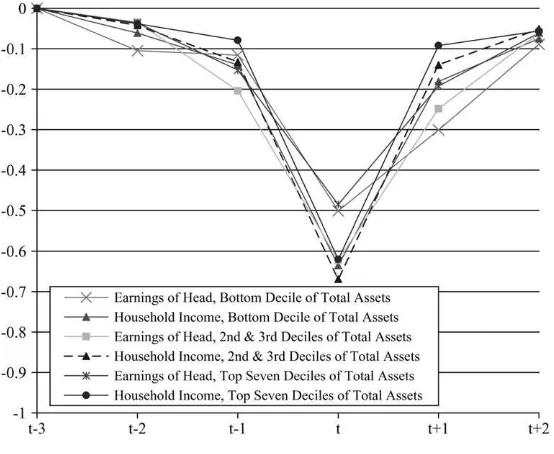
t+j, Xit is a vector of the same household demographics included in Equations 2 and 3, andhiis a household-specific effect. Estimates ofbjrepresent the effect of an unemployment spell in period t+j on an outcome in period t. Point estimates forbj are plotted in Figure 1, normalizing the first estimate to zero. Earnings for those at the bottom of the asset distribution start to fall prior to the period of the spell, suggesting that these spells are partly anticipated. Earnings fall by 12 percent from periodt-3 tot-1, and by 50 percent from periodt-3 tot. A similar pattern is evident for households at higher points in the asset distribution. For all asset groups, Figure 1 shows that both the earnings of the head and total household income recover substan-tially within two periods following the unemployment spell, which is not too surpris-ing given that, by construction, all spells end before the start of periodt+1. Earnings are only slightly lower two periods after the spell than three periods before. Thus, these spells do not appear to have a significant permanent effect on earnings and in-come for any of these asset groups. This finding is consistent with previous research that argues that unemployment spells that are not followed by subsequent displace-ment do not have a large long-term effect on earnings (Stevens 1997). It is important to note that even though the spells do not have a permanent effect, I cannot rule out that these households expect the effect to be permanent, and consumption and bor-rowing behavior depend on expectations about the permanence of these shocks.
V. Results
A. The Response of Unsecured Debt
To determine whether households borrow to maintain well-being in the presence of variable earnings, I estimate the responsiveness of unsecured debt to earnings 20. There are several potential explanations for why households with assets also hold unsecured debt, in-cluding transaction costs and hyperbolic discounting (Brito and Hartley 1995; Gross and Souleles 2002; Laibson, Repetto, and Tobacman 2003; Telyukova 2006).
shortfalls that result from transitory spells of unemployment (b
˘
from Equation 3). Rather than estimating the IV model in Equations 3 and 4 separately for different as-set groups, I estimate a single model that includes indicators specifying where the household falls in the total asset distribution, as well as interactions of these indicators with all other controls. Specifically, I separate households into four separate asset groups: those in the bottom decile (the baseline group), those in the second and third deciles, those in the fourth and fifth deciles, and those in the top half of the asset dis-tribution.21Alternative specifications examine households at different points in the dis-tribution of financial assets or asset-to-earnings ratios.
Table 3 reports IV estimates for the effect of unemployment-induced earnings var-iation on borrowing (using SIPP data) and consumption (using PSID data). The
Figure 1
The Long Run Effect of Unemployment on Income and Earnings by Asset Hold-ings (SIPP)
Notes: Data are from the 1996 and 2001 Panels of the SIPP. This figure plots point estimates from regressions of leads and lags of the unemployment indicator on household income and earnings of the head. These estimates represent changes in the outcome relative to period t-3. All models include the same controls as those listed in the notes to Table 3. See text for more details.
21. This model has four endogenous variables—the earnings change and this change interacted with indi-cators for each of the top three asset groups—and four instruments—the unemployment indicator and this indicator interacted with indicators for each of the top three asset groups. This approach yields precisely the same point estimates as running separate regressions for each asset subgroup.
Table 3
The Response of Unsecured Debt and Consumption to an Unemployment-Induced Earnings Loss (SIPP and PSID)
Dependent Variable, Change in
Asset Distribution Total Assets
Asset Distribution Financial Assets
Asset Distribution Asset-to-Earnings Ratio
Unsecured Debt Food
Food and Housing
Unsecured Debt Food
Food and Housing
Unsecured Debt Food
Food and Housing SIPP PSID PSID SIPP PSID PSID SIPP PSID PSID
(1) (2) (3) (4) (5) (6) (7) (8) (9)
Earnings change (b1) 0.051 0.091 0.319 0.058 0.079 0.313* 0.043 0.078 0.345
(0.050) (0.074) (0.195) (0.050) (0.064) (0.134) (0.051) (0.078) (0.226) Earnings change x 2nd and 3rd
deciles of asset distribution (b2)
-0.185* -0.024 -0.203 -0.172* -0.097 -0.291 -0.173* -0.016 -0.235 (0.081) (0.080) (0.201) (0.077) (0.074) (0.156) (0.074) (0.082) (0.230) Earnings change x 4th and 5th
deciles of asset distribution (b3)
-0.042 -0.084 -0.291 -0.070 -0.009 -0.175 -0.028 -0.060 -0.269 (0.064) (0.077) (0.201) (0.067) (0.074) (0.150) (0.060) (0.081) (0.231) Earnings change x top half
of asset distribution (b4)
-0.031 -0.075 -0.286 -0.041 -0.059 -0.303* -0.023 -0.065 -0.325 (0.054) (0.078) (0.198) (0.054) (0.067) (0.137) (0.056) (0.082) (0.229) N 20,241 11,518 11,518 20,241 11,518 11,518 20,241 11,518 11,518
b1+b2 -0.134 0.067 0.116 -0.115 -0.018 0.022 -0.130 0.062 0.110
b1+b3 0.008 0.007 0.027 -0.012 0.071 0.138 0.015 0.018 0.076
b1+b4 0.019 0.016 0.032 0.017 0.020 0.010 0.020 0.014 0.020
b3-b2 0.143 -0.060 -0.089 0.103 0.089 0.116 0.145 -0.044 -0.034
b4-b2 0.154 -0.052 -0.084 0.131 0.038 -0.012 0.150 -0.049 -0.090
(continued)
Sulli
v
an
Table 3 (continued)
Dependent Variable, Change in
Asset Distribution: Total Assets
Asset Distribution: Financial Assets
Asset Distribution: Asset-to-Earnings Ratio
Unsecured Debt Food
Food and Housing
Unsecured Debt Food
Food and Housing
Unsecured Debt Food
Food and Housing SIPP PSID PSID SIPP PSID PSID SIPP PSID PSID
(1) (2) (3) (4) (5) (6) (7) (8) (9)
P-values from tests of linear restrictions:
H0:b1+b2¼0 0.033 0.030 0.019 0.048 0.619 0.785 0.015 0.023 0.014
H0:b1+b3¼0 0.831 0.736 0.572 0.789 0.052 0.041 0.636 0.466 0.120
H0:b1+b4¼0 0.338 0.536 0.368 0.397 0.328 0.735 0.392 0.616 0.605
H0:b3-b2¼0 0.055 0.112 0.203 0.158 0.092 0.269 0.020 0.238 0.612
H0:b4-b2¼0 0.020 0.199 0.169 0.032 0.364 0.887 0.010 0.208 0.130
Notes: The baseline group includes households in the bottom decile of the asst distribution. For the PSID results, the standard errors in parentheses are corrected for within household dependence. All results are weighted. * denotes significance at the 0.05 level. All of the models include a cubic in age, a second order polynomial in family size and number of children, indicators for educational attainment, race, change in family size, and change in marital status, an indicator for having high initial debt, controls for state-level unemployment insurance and bankruptcy laws, and year dummies. All models also include asset group indicators as well as these indicators fully interacted with all covariates. See text for more details.
400
The
Journal
of
Human
results in Column 1 provide evidence on the responsiveness of unsecured debt for households at different points in the distribution of total assets. The response of un-secured debt for households in the bottom decile,b1, is positive, suggesting that un-secured borrowing decreases with unemployment-induced earnings losses, although the point estimate is small and insignificant.22This estimate provides virtually no ev-idence that these very low-asset households—those with less than $762 in total assets (Table 2)—borrow during unemployment spells. In fact, I reject a one-sided test that borrowing increases by more than 3.2 cents for each dollar lost. The estimates ofb1 for those at the bottom of the distribution of financial assets (Column 4) or asset-to-earnings ratios (Column 7) provide very similar evidence. These credit markets do not appear to be a safety net for those at the very bottom of the asset distribution.23 For other low-asset households—those in the second and third deciles of total assets (Column 1)—unsecured debt responds significantly to a job loss, increasing by 13.4 cents (b1+b2) for each dollar of earnings lost due to unemployment (p-value ¼ 0.033). The results are very similar for households in these same deciles of the dis-tribution of financial assets (11.5 cents) or asset-to-earnings ratios (13.0 cents). The magnitude of this response is comparable to other common sources for supplement-ing earnsupplement-ings losses. For example, Dynarski and Gruber (1997) estimate that unem-ployment insurance supplements 7–22 cents of each dollar of lost earnings due to unemployment. They estimate additional earnings of the spouse (the added worker effect) to respond by 2–12 cents for each dollar lost.
In each case, the borrowing behavior for those in the second and third deciles is significantly different from that of the lowest asset group (b2). Moreover, in nearly all cases, I can reject the hypothesis that the borrowing behavior for this group is the same as any of the other asset groups. For example, the estimates indicate that these households borrow 15.4 cents (b4-b2) more per dollar lost than those in the top half of the total asset distribution (p-value¼0.020). There is little evidence that higher asset households borrow in response to an unemployment-induced earnings loss. B. Consumption and Components of Net Worth
The fact that borrowing does not change in response to unemployment spells for some households indicates that these households are either supplementing income via other sources or reducing consumption. Table 3 also presents estimates of the re-sponsiveness of consumption to unemployment-induced earnings for two measures of consumption that are observable in the PSID—food and food plus housing.24 The point estimates for those in the bottom decile suggest that food consumption falls by between 8 and 9 cents for each dollar of lost earnings, but these estimates are not statistically significant. For the combined measure of food plus housing 22. This might be the case if, for example, households file for bankruptcy during unemployment to reduce debt. 23. The point estimate for state UI generosity is positive and significant, but only for households in the second and third decile of the asset distribution. Among the bankruptcy controls only the coefficient on the indicator for whether a state has a homestead exemption is significant, and only for households in the second and third deciles. This point estimate indicates that these households that live in states with a homestead exemption in-crease their unsecured borrowing by more than those in states with an unlimited exemption.
24. Other than housing, the PSID consumption measures do not include durable goods, which are likely to be the most elastic component of expenditures. Dynarski and Gruber (1997) show that the response of du-rable goods to an unemployment spell is greater than that of food and housing.
consumption, the IV estimates show a larger response.25For those in the bottom dec-ile of financial assets (Column 6), food plus housing consumption falls by 31.3 cents for each dollar of earnings lost, and this estimates is significant.
For households with higher assets there is evidence that the consumption re-sponse is smaller—b2,b3, andb4are all negative—and some of these differences are significant (Column 6). There is some evidence that food and housing con-sumption falls during unemployment for those in the second and third deciles, but the magnitude of this response is just over a third of that for those in the bottom decile of total assets. In all cases the response of both food and food plus housing consumption is small (less than 3.3 cents per dollar lost) and insignificant for households in the top half of the asset distribution (b1+b4). Similar results are ev-ident for those in the fourth or fifth deciles, except when grouped by financial assets (Columns 5 and 6).
These results for consumption are consistent with a number of previous studies that have examined the responsiveness of consumption to unemployment. For example, Dynarski and Gruber (1997) also find that unemployment spells result in a reduction in consumption for some households, although they do not focus on very low-asset households. For a sample of households in the bottom 75 percent of the financial assets distribution, they find that food and housing consumption falls by 25.5 cents for each dollar of earnings lost. Browning and Crossley (2001) also report drops in expenditures during unemployment for a low-asset sample. Stephens (2001) shows that job displacements result in persistent drops in consumption.
As additional evidence on how households supplement unemployment-induced earnings shocks, I also examine the responsiveness of other components of net worth to these earnings shortfalls. In Table 4, Columns 1–3, I present IV estimates for three different components: unsecured debt, secured debt, and financial assets. As an alter-native specification, Columns 4–6 report estimates from a reduced form equation regressing changes in these outcomes on the unemployment spell indicator as well as the other controls that are included in the IV models. Total secured debt (Columns 2 and 5) is not noticeably responsive to unemployment-induced earnings variation for households above the bottom decile of the asset-to-earnings distribution, and it decreases (insignificantly) for low-asset households. Secured debt could decrease in response to a negative earnings shock if a household liquidates a secured asset rather than borrowing against it. For example, a household may sell their car to sup-plement lost earnings, resulting in a reduction in vehicle debt.
The results reported in Table 4 indicate that financial assets may play an important role for supplementing lost earnings for households in the top half of the asset-to-earnings distribution. The point estimates suggest that these households liquidate 18.8 cents worth of assets for each dollar drop in earnings, although this estimate is only marginally significant (p-value¼0.099). Other studies have provided evidence of dis-saving among the wealthy in response to anticipated variation in income. Flavin (1991) finds that 30 percent of an anticipated increase in income is saved in financial assets for 25. Although housing consumption, which for this group is mostly rent, is likely to be inelastic in the short run due to rental contracts and the fixed costs of moving, data from the PSID show that households that experience an unemployment spell are 1.5 times more likely to move than households that do not experi-ence a spell. Data on reasons for moving show that unemployed households are also more likely to move for the purpose of reducing rent than other households.
Table 4
The Response of Components of Net Worth to an Unemployment-Induced Earnings Loss (SIPP)
Asset Distribution: Asset-to-Earnings Ratio
IV Estimates OLS Estimates
Dependent Variable, Change in Unsecured Debt
Secured Debt
Financial Assets
Unsecured Debt
Secured Debt
Financial Assets
(1) (2) (3) (4) (5) (6)
Earnings change (b1) 0.043 0.599 0.006
(0.051) (0.446) (0.249) Earnings change x 2nd and 3rd deciles
of asset distribution (b2)
-0.173* -0.488 0.042 (0.074) (0.647) (0.362) Earnings change x 4th and 5th deciles
of asset distribution (b3)
-0.028 -0.705 0.053 (0.060) (0.528) (0.296) Earnings change x top half of asset
distribution (b4)
-0.023 -0.676 0.183 (0.056) (0.490) (0.274)
Unemployment indicator (b1) -454 -6,321 -61
(532) (4,699) (2,632) Unemployment indicator x 2nd and 3rd
deciles of asset distribution (b2)
1,568* 5,376 -347 (699) (6,180) (3,461) Unemployment indicator x 4th and 5th
deciles of asset distribution (b3)
228 7,892 -804 (711) (6,283) (3,519) Unemployment indicator x top half of
asset distribution (b4)
167 7,431 -2,652 (626) (5,538) (3,101)
N 20,241 20,241 20,241 20,241 20,241 20,241
(continued)
Sulli
v
an
Table 4 (continued)
Asset Distribution: Asset-to-Earnings Ratio
IV Estimates OLS Estimates
Dependent Variable, Change in Unsecured Debt
Secured Debt
Financial Assets
Unsecured Debt
Secured Debt
Financial Assets
(1) (2) (3) (4) (5) (6)
b1+b2 -0.130 0.110 0.048 1,114 -945 -408
b1+b3 0.015 -0.107 0.059 -226 1,571 -865
b1+b4 0.020 -0.077 0.188 -287 1,110 -2,713
b3-b2 0.145 -0.217 0.011 -1,340 2,516 -457
b4-b2 0.150 -0.187 0.141 -1,401 2,055 -2,305
P-values from tests of linear restrictions:
H0:b1+b2¼0 0.015 0.814 0.856 0.014 0.814 0.856
H0:b1+b3¼0 0.636 0.707 0.711 0.632 0.707 0.711
H0:b1+b4¼0 0.392 0.705 0.099 0.386 0.705 0.098
H0:b3-b2¼0 0.020 0.693 0.971 0.041 0.664 0.888
H0:b4-b2¼0 0.010 0.714 0.623 0.013 0.679 0.408
Notes: The unsecured debt results in Column 1 are from Column 7 of Table 3. Secured debt includes auto loans, mortgage debt, and other asset-backed loans. See the notes to Table 3 for a list of additional controls included in these models. * denotes significance at the 0.05 level.
404
The
Journal
of
Human
wealthy households. Alessie and Lusardi (1997), who provide similar estimates for a high-income sample, suggest that 30 to 50 percent goes into financial assets. The results in Table 4 show little evidence that financial assets respond to these income shocks for households in the bottom half of the asset-to-earnings distribution.
The OLS estimates are consistent with the IV estimates. Again, we see that unse-cured debt (Column 4) does not respond to these unemployment spells for those in the bottom decile of the asset-to-earnings distribution. For those in the second and third deciles, an unemployment spell results in an increase in unsecured debt of $1,114 (p-value 0.014), and this response is significantly different from that of both very low-asset and higher asset households. As with the IV estimates, the OLS esti-mates provide little evidence that households are using secured debt in response to these unemployment spells, but there is some evidence that wealthy households liq-uidate assets during unemployment.
VI. Why Very Low-Asset Households Do Not Borrow
There are a number of potential reasons why very low-asset house-holds do not borrow. For example, these househouse-holds may not have an incentive to borrow if they supplement the shortfall via other income sources such as public or private transfers. Previous research, however, shows that this is unlikely in the case of unemployment shocks. Results from Dynarski and Gruber (1997) suggest that government transfers, other than UI, play a very small role in supplementing unem-ployment-induced earnings losses, and they argue that for many households UI does not provide enough liquidity to maintain consumption during unemployment. In ad-dition, transfers such as public assistance are not likely to play an important role in my analysis, because all household heads in my sample have a strong attachment to the labor force. Also, Bentolila and Ichino (2008) provide evidence that family trans-fers are not an important source of insurance for U.S. households. Moreover, if very low-asset households are fully able to supplement lost earnings via other sources of income, such as public or private transfers, then we would not expect consumption to fall. The results in Table 3, however, indicate that consumption is sensitive to these transitory earnings shocks, suggesting that these households do not have sufficient access to public and private transfers to smooth consumption fully over transitory earnings variation.
That these very low-asset households do not borrow and that consumption falls during a transitory income shortfall is consistent with a model where these house-holds face frictions in credit markets. Descriptive evidence on access to credit card debt—a major component of unsecured debt—from the SCF indicates that very low-asset households have limited access to these markets. Fewer than one in five of these households have a credit card. Moreover, the average total credit limit for those households with cards is only $1,958, and net of outstanding balances, their available credit is less than $800.26 Thus, few very low-asset households have access to enough liquidity via credit cards to offset even a small fraction of the average earn-ings shortfall from unemployment of about $10,000 (Table 1). Half of all very
low-26. These statistics are based on the author’s calculations using the 1995 SCF.
asset households that have applied for credit have been denied within the past five years, and nearly a third report that they did not apply for credit because they expected to be turned down. Moreover, from Table 2 we see that 43 percent have no unsecured debt at all. Other studies have shown evidence of frictions in unsecured credit markets. Gross and Souleles (2002) draw from evidence that households re-spond to changes in the credit limit on credit cards to conclude that many households are constrained from borrowing with credit cards.27
Even if these households have access to credit, it may not be optimal for them to borrow to smooth transitory shocks if the borrowing rate is too high. In other words, the utility loss that results from a drop in consumption may not be sufficient to justify borrowing at high rates. Those that do maintain balances on their credit cards pay interest rates of about 15 percent. These households may face constraints in unse-cured credit markets in that they can only borrow at prohibitively high rates. Davis, Kubler, and Willen (2006) demonstrate that high borrowing costs discourage con-sumption smoothing through credit markets.
While the evidence presented thus far suggests that very low-asset households do not borrow due to constraints in unsecured credit markets, several other possible explanations cannot be ruled out. If these households experience unemployment spells that have a permanent effect on earnings, then these households have an incentive to reduce consumption rather than borrow to maintain well-being. Thus, the assumption that the earnings shocks identified in the data are temporary is critical for determining why, in response to these shocks, very low-asset households do not borrow, and why consumption falls. To some extent, I mitigate complications with more permanent spells of unemployment by focusing on households that work again and do not expe-rience an unemployment spell the year following the initial job loss. This restricts at-tention to unemployment spells that are observed to be temporary, and the evidence in Figure 1 suggests that the spells have a temporary effect on earnings. However, house-holds may expect these temporary spells to be permanent, and consumption and bor-rowing behavior depend on expectations about the permanence of these shocks.
Precautionary motives also might affect the estimates presented earlier if house-holds are risk averse and unemployment shocks generate greater uncertainty about future earnings. Carroll and Samwick (1998) find strong evidence that some house-holds save for precautionary reasons. For these motives to explain the findings in this study, however, the unemployment shocks need to generate greater uncertainty for very low-asset households than for other households.28 However, evidence from
27. The literature on liquidity constraints is somewhat in agreement that at least some households face binding constraints, but there is little consensus on how to identify which households are constrained. Sev-eral studies have used the initial level of wealth to identify constrained households (Zeldes 1989; Dynarski and Gruber 1997; Souleles 1999; Browning and Crossley 2001; Hurst and Stafford 2004). Other studies use self-reports of constraints (Jappelli 1990; Cox and Jappelli 1993; Jappelli, Pischke, and Souleles 1998). Engelhardt (1996) notes that households transitioning from renting to owning face a down payment con-straint. Also, Garcia, Lusardi, and Ng (1997) model the probability that a household is constrained as a function of social and economic factors beyond just income and assets.
Carroll, Dynan, and Krane (2003) suggests that the role of precautionary motives is small for very low-asset households.29
VII. Other Samples and Robustness
I also examine whether borrowing behavior is different for certain subgroups, such as young or less-educated households. The results in Table 5 show evidence that for these groups the response is somewhat larger than those reported earlier. However, there is evidence of heterogeneity in the responsiveness of borrow-ing across asset holdborrow-ings. Among households in the second and third deciles of the asset distribution with heads that do not have a high school degree, unsecured bor-rowing increases by 46.6 cents for each dollar of earnings lost due to unemployment. The response is larger (53.8) and statistically significant when looking at these dec-iles of the distribution of asset-to-earnings ratios, but the response is much smaller for those in these deciles of the distribution of financial assets. High school dropouts with very low-assets show no evidence of borrowing in response to an earnings shock, and in some cases (Column 7), I can reject that the responsiveness of borrow-ing is the same across asset holdborrow-ings. The results for a sample of young households are similar, although less precise. I also verify that the results for a sample of only mar-ried families (not reported) do not differ noticeably from those reported in Table 3.
The data suggest that one-third of all households do not maintain any unsecured debt (Table 2). These households may be systematically different from households with nonzero unsecured debt for several reasons including unobserved borrowing constraints, risk aversion, or low discount rates. To examine the degree to which these households without any initial unsecured debt influence the results, I examine the borrowing behavior for households with positive debt initially. The results in Col-umns 3, 6, and 9 of Table 5 are consistent with those reported in Table 3. Very low-asset households with positive ex ante debt do not borrow in response to the earnings shock, but there is evidence that other low-asset households do borrow. In some cases (Columns 3 and 9) the responses for households in the second and third deciles of the asset distribution are noticeably larger than those reported in Table 3. Again, we see no evidence that higher asset households borrow during unemployment. For the sample of households with zero initial unsecured debt (not reported), there is little evidence that borrowing responds to the earnings shortfalls regardless of the house-hold’s asset holdings. This suggests that ex ante debt may be a proxy for access to these markets.
Other specifications are estimated to determine whether the results are sensitive to assumptions about the functional form of the borrowing equation, such as nonlinear-ities in the distribution of changes in borrowing;DDi¼0 for more than a fifth of all households (Table 2). Results for a sample of households that have nonzero changes 29. Other factors, such as differences in nonseparability across asset holdings, may explain the findings in Section V. For example, there may be differences across these groups with respect to work related expenses, risk aversion, or preferences for leisure. Also, unobserved factors that are correlated with having few assets may also explain why these households do not borrow. For example, these very low-asset households may exhibit hyperbolic discounting that may lead them to borrow up to their limits prior to an earnings shock (Laibson, Repetto, and Tobacman 2003).
Table 5
The Response of Unsecured Debt for Other Samples (SIPP)
Asset Distribution:
Earnings change (b1) 0.090 0.014 0.037 -0.086 0.086 0.055 0.108 0.132 0.052 (0.110) (0.922) (0.079) (0.101) (0.222) (0.095) (0.119) (0.298) (0.078) Earnings change x 2nd and 3rd
deciles of asset distribution (b2)
-0.556 -0.352 -0.250* 0.015 -0.278 -0.175 -0.646* -0.360 -0.287* (0.309) (1.007) (0.108) (0.164) (0.354) (0.121) (0.251) (0.332) (0.122) Earnings change x 4th and 5th
deciles of asset distribution (b3)
-0.223 3.982 -0.015 0.057 -0.311 -0.093 -0.064 -0.294 -0.062 (0.164) (5.575) (0.089) (0.164) (0.255) (0.107) (0.222) (0.387) (0.093) Earnings change x top half of asset
distribution (b4)
-0.045 -0.065 0.004 0.023 0.038 -0.025 -0.090 -0.080 -0.011 (0.161) (1.058) (0.087) (0.224) (0.519) (0.099) (0.166) (0.447) (0.084) N 1,894 1,365 13,525 1,894 1,365 13,525 1,894 1,365 13,525
b1+b2 -0.466 -0.338 -0.213 -0.071 -0.192 -0.120 -0.538 -0.228 -0.235
b1+b3 -0.134 3.996 0.022 -0.029 -0.225 -0.038 0.044 -0.162 -0.010
b1+b4 0.045 -0.051 0.041 -0.063 0.124 0.030 0.018 0.052 0.041
b3-b2 0.333 4.334 0.235 0.042 -0.033 0.083 0.581 0.066 0.225
b4-b2 0.511 0.287 0.254 0.008 0.316 0.150 0.555 0.280 0.276
P-values from tests of linear restrictions:
H0:b1+b2¼0 0.106 0.408 0.004 0.583 0.482 0.112 0.015 0.114 0.012
H0:b1+b3¼0 0.272 0.467 0.603 0.821 0.077 0.461 0.816 0.502 0.844
H0:b1+b4¼0 0.699 0.920 0.269 0.752 0.793 0.323 0.880 0.866 0.184
H0:b3-b2¼0 0.288 0.431 0.006 0.818 0.914 0.366 0.045 0.815 0.034
H0:b4-b2¼0 0.101 0.661 0.002 0.972 0.560 0.066 0.026 0.410 0.005
Notes: In each model, the dependent variable is the change in unsecured debt. Deciles are based on the overall asset distribution, so the decile cutoffs are the same as those used in Table 3. All models include the same controls as those listed in the notes to Table 3. * denotes significance at the 0.05 level.