The Socioeconomic Gradient of
Child Development: Cross- Sectional
Evidence from Children 6–42
Months in Bogota
Marta Rubio- Codina, Orazio Attanasio, Costas Meghir,
Natalia Varela, Sally Grantham- McGregor
Rubio- Codina et al.abstract
We study the socioeconomic gradient of child development on a sample of low- and middle- income children aged 6–42 months in Bogota using the Bayley Scales of Infant and Toddler Development. We fi nd an average difference of 0.53, 0.42, and 0.49 standard deviations (SD) in cognition, receptive, and expressive language respectively, between children in the top and bottom quartile of the wealth distribution. These gaps increase substantially to 0.81 SD (cognition), 0.76 SD (receptive language), and 0.68 SD (expressive language) for children aged 31–42 months. These robust fi ndings can inform the design and targeting of interventions promoting early childhood development.
Marta Rubio- Codina is a senior research economist at the Centre for the Evaluation of Development Policies (EDePo) at the Institute for Fiscal Studies and a senior economist at the Inter- American Development Bank. Orazio Attanasio is a professor of economics at the Department of Economics at University College London and a research fellow and codirector of EDePo at the Institute for Fiscal Studies. Costas Meghir is a professor of economics at the Department of Economics at Yale University and a research fellow at the Institute for Fiscal Studies. Natalia Varela is a doctoral candidate at Université Laval. Sally Grantham- McGregor is emerita pro-fessor of international child health at the Institute of Child Health at University College London. The opinions expressed herein are those of the authors and not necessarily of the institutions they represent. This research would not have been possible without the outstanding work of Pablo Muñoz, Mara Minski, Belén Gómez, Juan Fernando Trujillo and Hanner Sánchez in the fi eld; and funding from the Inter- American Development Bank for data collection. The authors are grateful to the BibloRed network of libraries, Jardines Sociales del Distrito de Bogota, and aeioTu centers for lending us their facilities. The authors thank Camila Fernández, researchers at EDePo, and two anonymous referees for useful comments and suggestions; and José Guerra for research assistance. Rubio- Codina’s research time was fi nanced by the Leverhulme Trust Early Career Fellowship ECF/2008/0170 on “CCTs, Child Care and Child Development.” Attanasio’s research time was partially fi nanced by the European Research Council Advanced Grants 249612 on “Exiting Long Run Poverty: The Determinants of Asset Accumulation in Developing Countries” and by the ESRC Professorial Fellowship ES/K010700/1 on “The Accumulation of Human Capital in Developing Countries.” Rubio- Codina, Attanasio, and Meghir acknowledge fi nancial support to research time from Grand Challenges Canada. All errors are the authors’ own. The data used in this article can be obtained beginning November 2015 through October 2018 from Marta Rubio- Codina. Correspondence to: Marta Rubio- Codina, Institute for Fiscal Studies, 7 Ridgmount Street, London WC1E 7AE, UK. Email: marta_r@ifs.org.uk. Telephone: +44 20 7291 4800.
[Submitted January 2013; accepted March 2014]
ISSN 0022- 166X E- ISSN 1548- 8004 © 2015 by the Board of Regents of the University of Wisconsin System
Rubio- Codina et al. 465
I. Introduction
In low- and middle- income countries, an estimated 219 million (39 percent) children younger than age fi ve fail to reach their developmental potential due to exposure to risk factors such as illness, nutritional defi ciencies, and less- responsive parents—all of which are associated to poverty (Grantham- McGregor et al. 2007). These factors affect cognitive abilities beyond the effect of genetics (Hackman and Farah 2009) and generate developmental delays that are diffi cult to compensate later on in life given the plasticity of the brain in early childhood (Shonkoff 2010). Lower school readiness and performance, lower employability and earnings, and worse adult health and well- being, are among the long- term consequences of exposure to these factors (see Almond and Currie 2010 and references therein).
Hence, low early childhood development levels may not only undermine the ex-pected social and economic benefi ts of public (governmental) and private (parental) investments in children’s health and education later in life but also reduce the quality of the human resources available in the labor market, thus affecting the aggregate economy (Naudeau et al. 2011). Given the high private and public returns of improved outcomes in the early years, understanding when and why disadvantages in child de-velopment start is critical to the design of well- targeted, timely interventions.
The positive association between poverty and socioeconomic status (SES)—as measured by income, wealth, or parental education—on child health and development has been well documented in Western countries (Blau 1999; Bradley and Corwyn 2002; Aughinbaugh and Gittleman 2003), the gradient in health widening as children get older (Case, Lubotsky, and Paxson 2002).
An increasing number of studies are documenting similar patterns in developing countries. Paxson and Schady (2007) fi nds a difference close to two standard devia-tions (SD) on receptive language—measured on the Spanish version of the Peabody Picture Vocabulary Test (PPVT)—between children three to six years old in families in the 90th and 10th percentile of the wealth distribution in poor rural Ecuador.
Ma-cours, Schady, and Vakis (2012) fi nds qualitatively similar gaps on the PPVT for chil-dren three to seven years old in highly disadvantaged communities in rural Nicaragua as do Bernal and Van Der Werf (2011) when comparing children three to ten years old in the lowest and highest third of the wealth distribution for a Colombia- wide representative sample. This gap is largest among children in urban areas, and more so for children aged four and a half to eight and a half.
Outside Latin America, Ghuman et al. (2005) reports a negative association be-tween household assets and receptive language for low- income children younger than age three in the Philippines. More recently, Fernald et al. (2011) assesses a nationally representative sample of children three to six years old in Madagascar on a range of cognitive and language measures and fi nds that children from families in the top wealth quintile or whose mothers had secondary education perform signifi cantly bet-ter. These differences double between age three and six. In line with this evidence are the fi ndings from two parallel World Bank studies on three- to fi ve- year- olds in rural Mozambique (Bruns et al. 2010) and Cambodia (Filmer and Naudeau 2010).
op-The Journal of Human Resources 466
posed to a comprehensive range of developmental functions. Finally, little is known to date about the gap before three years of age, except for recent works by Hamadani et al. (2014) and Fernald et al. (2012). The fi rst study collects high- quality measures of cognition—the Bayley Scales of Infant Development (BSID- II) and the Wechsler Preschool and Primary Scale of Intelligence (WPPSI- II)—for a panel of poor children in rural Bangladesh over a period of fi ve years since birth, and shows that the cognitive gap associated with poverty starts at seven months. Fernald et al. (2012) documents SES gaps on child development for under two- year-olds in rural India, Indonesia, Peru, and Senegal. They, however, use a measure based on maternal reports—the Ex-tended Ages and Stages Questionnaire(EASQ), which is thus likely to be less reliable. In this paper, we study a representative sample of children aged 6–42 months in the lowest three (out of six) socioeconomic strata in the city of Bogota, Colombia. Eighty-fi ve percent of the city’s population lives in these strata. We construct an index of house-hold wealth and estimate the SES gradient in child development, measured using all scales of the latest version of the Bayley Scales of Infant and Toddler Development (Bayley- III): cognitive, receptive language, expressive language, fi ne motor, gross mo-tor, and socioemotional. The Bayley- III offers a complete picture of a child’s develop-mental level by direct observation of their abilities and is currently considered the gold standard for the assessment of children up to 36 months by many (Fernald et al. 2009).
Hence, our study contributes to the existing literature by describing the develop-mental profi le of children at very early ages in low- and middle- income groups in a typical Latin American urban environment, using one of the highest quality mea-sures available. This allows studying any differences in the SES gap with age across developmental domains, which in turn can inform the design and timing of effective interventions.
We fi nd sizeable average SES differences on cognition (0.53 SD), receptive language (0.42 SD), and expressive language (0.49 SD) between children in the top and bottom quartile of the household wealth distribution. The SES gap is about half the size for fi ne motor and socioemotional development, at 0.26 SD and 0.27 SD respectively, and not signifi cant in gross motor skills. In line with the existing evidence, these gaps (except receptive language) are statistically signifi cant even among the youngest in the sample (6–18 months) at conventional levels, and at the 10 percent for cognition. Similarly, as reported elsewhere, these differences increase with age, reaching levels of 0.81 SD (cognition), 0.76 SD (receptive language), 0.68 SD (expressive language), 0.40 SD (fi ne motor), and 0.38 SD (socioemotional) for children aged 31–42 months. Finally, we fi nd that the SES gap persists after controlling for other factors likely correlated with wealth, including maternal education, and is robust to a number of alternative specifi cations.
The paper is organized as follows. The next section describes the study design, the sample, and the data. In Section III, we estimate the SES gap by age and developmen-tal domain. Section IV presents a number of robustness tests and Section V concludes.
II. Study Design: Sample and Data
Rubio- Codina et al. 467
given the socioeconomic stratifi cation fi rst introduced in Bogota in the 1980s as a mechanism to target the subsidization of basic public services (such as drinking water, electricity, and gas). Following the 1994 law of Public Services, the Department for National Planning classifi ed entire blocks into six strata—“estratos”—according to their location and quality of infrastructure and housing. This scheme is, in principle, revised every fi ve years. For our sampling exercise, we combined data from the 2005 Census and the 2001 Cadastre, which classifi ed 12.6 percent of all residential blocks in Bogota as estrato 1 (E1), 38.9 percent as estrato 2 (E2), 36.6 percent as estrato 3 (E3), 6.9 percent as estrato 4 (E4), 2.9 percent as estrato 5 (E5), and the remaining 2.2 percent residential blocks as estrato 6 (E6).1
In practice, however, it is extremely diffi cult to contact and obtain participation consent from the higher strata, who often live in restricted access apartment blocks and compounds. For this reason, at the beginning of the project, we decided to exclude the wealthiest two sectors (E5 and E6) and focus on the fi rst four estratos. These represent about 95 percent of the population of the city. We designed the original study sample to be balanced across E1 to E4 and eight- month range age groups, with 90 children in each stratum- age cell, for a total of 1,440 children in 240 blocks.
Data were collected in three stages. First, once neighborhoods and blocks within them were selected, we visited all households in a block to identify those with chil-dren aged 6–42 months.2 Next, trained interviewers carried out a household survey
on a random subsample of these children to collect: basic household socioeconomic information (such as demographic composition, education, and employment for all household members, dwelling characteristics, and assets); information on the child’s nutritional status (such as birth weight and gestational age); formal and informal child-care arrangements; and the number of play activities and play materials using UNI-CEF’s Family Care Indicator (Frongillo, Sywulka, and Kariger 2013).
In a third and fi nal stage, the Bayley- III test was administered in the presence of the mother/main caregiver by trained psychologists (testers) in the library or public childcare center closest to the child’s home. Height and weight of both mother and child were also collected. The online Appendixes 1 and 2 (associated with this article at http://uwpress.wisc.edu/journals) provide more details on sampling, data collection procedures, and the instruments used.
A. Analysis Sample
Data collection took place between March and August 2011 on a sample of 1,533 children aged 6–42 months in 497 blocks mostly in estratos 1 to 3 (more than double the number of blocks originally planned).. The Bayley- III test was administered to
1,330 (86.8 percent) of the children for whom we have a household survey. These children constitute our sample of analysis. Table A1 in the online appendix reports summary statistics for this sample by estrato and shows sample balance in age and
1. See DANE (2011) for more details. More recently, the distribution seems to have shifted slightly to the right: 8.1 percent of all residential blocks are classifi ed as E1, 37.3 percent as E2, 38.2 percent as E3, 11.3 percent as E4, 2.1 percent as E5, and the remaining 2.7 percent as E6.
The Journal of Human Resources 468
gender, as well as a positive relationship between estrato and standard measures of household SES.
Geographically, the sample spans all Bogota and is, a priori, representative of ap-proximately the 85 percent of the city population that lives in these estratos. A few considerations are, however, in order. First, we have very few children from E4. As we discuss in the online appendix, soon after the start of fi eld activities, it was clear that E4 households were extremely reluctant to participate in the survey, mostly because of apparent mistrust. To compensate for the loss of children in E4, we increased the number of children in E1 and E2 by 90 each. In addition, mindful of the larger degree of heterogeneity in SES to be found in E3, we oversampled this estrato, adding 180 children. Second, refusals to participate in the study were more frequent in E1 than in E2 and E3, possibly also due to higher mistrust among those most vulnerable.
Hence, while we use estrato as a sampling device to ensure we obtain suffi cient observations, we will consider household wealth as our variable of interest in the analysis. Findings are robust to using sampling weights, an issue we return to in Sec-tion IV.
B. Construction of a Household Wealth Index
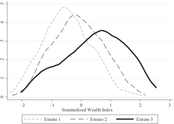
Panel III in Table A1 reports household characteristics by estrato. While there is a strong correlation between estrato of residence and household economic well- being, there is also substantial within- estrato heterogeneity. This is illustrated by the ample geographical dispersion of E3 across the city, from more peripheral areas neighboring E2 to very central areas surrounding E4 and E5, with many more services and ameni-ties (see Appendix Figure A1), and by the variance in the distribution of observables within estrato (Table A1). We formally assess the level of heterogeneity within estratos by constructing a household wealth index using principal component analysis on data on assets and dwelling characteristics (Filmer and Scott 2012).
Rubio- Codina et al. 469
follows, we will use the household wealth index to investigate the SES gradients. In particular, we will compare developmental outcomes for children living in households in the bottom quartile of the wealth index distribution (Q1) with households living in subsequent quartiles (Q2, Q3, and Q4).
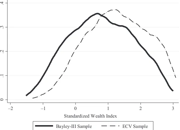
We investigate the wealth- representativeness of our sample relative to the overall population of Bogota by estimating a new wealth index using households in Bogota from a nationally representative sociodemographic survey, the 2010 Encuesta de Calidad de Vida(ECV), and the set of wealth- related variables available in both data sets.3 We then use the estimated factor loadings to compute a new wealth index for
both the ECV and our sample. Figure 2 plots the density of this index in both samples.
As our sample excludes households living in E4 to E6, the density of the wealth index is shifted to the left relative to that in the ECV. However, and perhaps surprisingly, the support of our sample is almost as large as that of the ECV: The largest value of the wealth index in our sample corresponds roughly to the 98th percentile of the ECV,
indicating large wealth- representativeness.
Table 1 reports summary statistics for the study sample by quartile of the distribu-tion of the household wealth index. As shown, the distribudistribu-tion of age and sex is well balanced across quartiles. However, not surprisingly, maternal age and employment and parental education increase with household SES. Panel III lists household size alongside the set of variables used in the construction of the wealth index. These
3. These are: car, fridge, microwave, washer, boiler, computer, DVD, stereo, console, Internet, shared kitchen, shared bathroom, more than one bathroom, quality fl oors, and crowding index.
0
.1
.2
.3
.4
.5
–2 –1 0 1 2 3
Standardized Wealth Index
Estrato 1 Estrato 2 Estrato 3
Figure 1
The Journal of Human Resources 470
offer a good characterization of economic well- being in the sample. Over 90 percent of dwellings in the top quartile have quality fl ooring, a fridge, a washing machine, a computer; 99.4 percent have external windows. The situation is very different at the opposite end of the distribution: Only 39.6 percent of the dwellings have quality fl ooring, 31.8 percent have a fridge, 11.7 percent a washing machine, and 4.2 per-cent and 3 perper-cent have a computer and Internet access; 31.2 perper-cent lack external windows. The level of stimulation in the home (FCI scores in Panel IV) and having a child minder also are correlated positively with the household SES.
C. Child Development Outcomes: Externally Versus Internally Standardized Scores
We assessed child development using the cognitive, receptive language, expressive language, fi ne motor, gross motor, and socioemotional scales of the third version of the Bayley Scales of Infant and Toddler Development (Bayley- III, Bayley 2006).
The fi rst fi ve scales consist of a series of tasks (items) of increasing diffi culty that the child has to perform. The child scores one for each item correctly executed and zero otherwise. The socioemotional scale consists of a maximum (depending on the child’s age) of 35 fi ve- point frequency rating questions responded by the mother/ main caregiver. The online Appendix 3 provides more details on the test, training, and administration.
Figure 2
Distribution of the Household Wealth Index in Our Sample (Bayley- III) and in the ECV Sample
0
.1
.2
.3
.4
–2 –1 0 1 2 3
Standardized Wealth Index
Rubio- Codina et al. 471
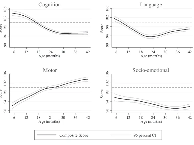
For each scale, the raw score is the sum of all correct responses. Raw scores are adjusted by age and diffi culty level in a nonlinear fashion to produce the composite scores, constructed to have a mean of 100 and a SD of 15 at every month- of- age. The norms (weights) used to construct composite scores are based on the reference popula-tion on which the test was standardized: a representative sample of 1,700 children in the United States. Also, the receptive and expressive language and the fi ne and gross motor subscales are combined to produce a single language and motor scale, respec-tively. Working with externally standardized scores is useful as it allows comparing scores within and across populations and across scales. However, some anomalies in the distribution of the composite scores by age suggest that the external norms used to standardize the Bayley- III may not be appropriate for our sample.
In Figure 3, we plot kernel estimates of average cognitive, language, motor, and socio-emotional composite scores against age (in months), along with 95 percent confi dence intervals. Given that composite scores are constructed to have a mean of 100 points at every month- of- age, we would expect the nonparametric regression line to be fl at around 100. Instead, we observe nonlinear relationships between the scores and age.
To an extent, the negative age gradients—this is to say, the presumed delayin devel-opment with respect to the population of reference as the child ages—in cognition and language, and to a lesser degree, for socioemotional development, are to be expected given that we are working with a more deprived sample (representative of low- and middle- income groups in Bogota) than the sample for which the test was standard-ized (representative of all socioeconomic groups in the United States). However, the 12- point increase in motor development over the age range and the four- point increase in language scores from 22 to 42 months are unusual. These unexpected relationships with age could be explained by cultural differences between the standardized and study populations, as well as by problems with translation.4 Similarly, they could also explain
the early advantage children in the sample seem to have in cognition and language. Table A2 in the online appendix reports means and SDs of the composite scores by quartile of the household wealth index and 12- month age groups. By age, the evolu-tion of the scores for each wealth quartile displays similar patterns to those observed in Figure 3 for the entire sample. The SDs are smaller than the expected 15 points in the standardized population and decrease with age, particularly for cognition. The chang-ing SD with age and the relation of the mean scores to age suggest the unsuitability of external norms and highlight the need to use internally standardized scores that adjust for age so as to allow comparisons.
Hence, as commonly done with developing country data, our analysis will focus on within- country comparisons between SES groups and use internally standardized scores. Often the standardization is done by dividing the sample into the smallest possible age groups—ideally monthly, given how sensitive developmental milestones are to age in the early years—but guaranteeing enough observations per group, and computing z- scores within age groups. (Subtract the months- of- age- specifi c mean of the raw score and divide by the months- of- age- specifi c SD.) (See Fernald et al. 2011, for example.)
472
Table 1
Mean Sample Characteristics by Wealth Quartile
Quartile 1 Quartile 2 Quartile 3 Quartile 4
I Child characteristics
Age (months) 23.709 (10.446) 23.666 (10.924) 24.294 (10.130) 24.205 (9.983)
Female =1 0.511 0.469 0.552 0.440
Premature (gestational age < 37 weeks) =1 0.162 0.122 0.152 0.184
Birth weight in grams 3,040.6 (484.7) 3,012.8 (536.3) 3,034.6 (506.6) 3,062.3 (536.6)
Stunted (z- height- for- age < –2 SD) =1 0.229 0.204 0.145 0.127
Firstborn =1 0.417 0.501 0.524 0.572
II Parental characteristics
Age mother 25.302 (6.185) 26.040 (6.122) 27.565 (7.041) 28.895 (6.673)
Education years mother 8.319 (3.251) 9.865 (2.749) 10.517 (2.988) 12.448 (3.110)
Mother has more than secondary education =1 0.106 0.176 0.329 0.607
Mother works (paid or unpaid) =1 0.442 0.437 0.565 0.619
Mother gave birth before age 18 =1 0.186 0.134 0.136 0.075
Education years father 6.846 (3.321) 8.042 (3.445) 8.977 (3.545) 9.653 (4.676)
Father has more than secondary education =1 0.059 0.167 0.270 0.493
Father deceased/no longer in household =1 0.291 0.340 0.315 0.334
III Household characteristics
Household size 4.444 (1.792) 4.687 (1.638) 4.736 (1.545) 4.771 (1.340)
Grandmother lives in household =1 0.147 0.272 0.285 0.370
Crowding (people per room)a 3.053 (1.279) 1.852 (0.819) 1.388 (0.633) 1.054 (0.380)
Quality fl oors (tiles, carpet, wood) a =1 0.396 0.618 0.824 0.952
External windowsa =1 0.688 0.881 0.942 0.994
Shared kitchena =1 0.417 0.212 0.106 0.045
Shared bathrooma =1 0.574 0.272 0.088 0.027
473
Cara =1 0.003 0.012 0.064 0.419
Fridgea =1 0.318 0.749 0.906 0.994
Microwavea =1 0.015 0.084 0.239 0.572
Washing machinea =1 0.117 0.475 0.794 0.961
Boilera =1 0.078 0.212 0.458 0.804
Computera =1 0.042 0.122 0.573 0.907
Smartphonea =1 0.015 0.021 0.079 0.295
Flat TVa =1 0.054 0.131 0.206 0.575
Home theatrea =1 0.009 0.057 0.091 0.235
DVDa =1 0.453 0.707 0.791 0.934
Stereoa =1 0.309 0.606 0.721 0.831
Games consolea =1 0.039 0.104 0.094 0.259
Interneta =1 0.030 0.131 0.382 0.795
Garagea =1 0.000 0.036 0.133 0.485
IV Level home stimulation
Books and newpapers (FCI Score) 1.574 (1.768) 2.376 (1.860) 2.897 (1.960) 3.780 (1.935) Play materials (FCI Score) 3.742 (2.105) 4.391 (2.221) 4.942 (2.229) 5.979 (2.269) Play activities (FCI Score) 3.904 (1.710) 4.107 (1.629) 4.524 (1.745) 4.991 (1.565)
V Childcare arrangements
Childcare center attendance =1 0.267 0.313 0.324 0.340
Care minder =1 0.426 0.499 0.552 0.608
The Journal of Human Resources 474
We follow this approach but compute internal z- scores in a more fl exible form in order to replicate as closely as possible the way in which the Bayley- III constructs composite scores while taking into account our limited sample size. In particular, in-stead of using months- of- age- specifi c means and SDs, we estimate age- conditional means and SDs using regression methods as described in the online Appendix 4.5 This
procedure is less sensitive to outliers and small sample sizes within age category. As expected, the substantive results that compare across wealth groups are unaffected by this procedure or the use of composite scores. Section IV provides more details on this.
III. SES Gap by Developmental Domain
We start by exploring the timing of the SES gap by developmental domain and how it varies with age nonparametrically. The graphs in Figure 4 plot kernel- weighted local polynomial regressions of the cognitive, receptive and expres-sive language, fi ne and gross motor, and socioemotional internally standardized scores on age for the lowest (Q1) and highest (Q4) quartiles of the distribution of household wealth, along with 95 percent confi dence intervals.
5. Bayley-III composite scores are a nonlinear function of raw scores where: (i) items administered in younger ages are given more weight, and (ii) months-of-age are lumped together until the age of 36 months, and in larger intervals thereafter.
Rubio-
The Journal of Human Resources 476
The top left graph in Figure 4 displays a remarkable gap in cognition, signifi cant from at least as early as 12–13 months of age, and reaching levels of almost one SD by 42 months of age.6 The gap increases throughout the entire age range, given that
children in the bottom quartile exhibit a negative age gradient (cumulative delay with age), whereas the age gradient for children in households in the top quartile is positive.
Similarly, the next two graphs show an age- increasing SES gap in receptive and expressive language that becomes signifi cant earlier—at around ten and eight months of age, respectively. However, from about 18–24 months of age, the gap becomes statistically insignifi cant. Note that this age range coincides with the “dip” in language scores shown in Figure 3, which may partly be attributable to inaccuracy in the measurement of language skills at these early ages using the Bayley- III as translated. Note also that the scores and gap in receptive language vary more con-sistently with age than the expressive language ones. This pattern may be related to the fact that the development of receptive language skills precedes that of expressive language skills.
The bottom graphs show that, while fi ne motor scores for children in the richest 25 percent of the wealth distribution are always higher than for those in the poorest 25 percent, gross motor scores are higher for the poorest children until 20 months of age. These differences are not statistically signifi cant. Finally, the gap in socioemo-tional development is considerably smaller than that in cognitive or language devel-opment over the age interval we consider, attaining a maximum value of 0.4 by 42 months and becoming statistically signifi cant much later, at around 32 months of age.
Next, we use a parametric framework to quantify the size of the SES gap on child development. We compare mean developmental levels for children in households in different quartiles of the distribution of the household wealth index, by estimating, for each developmental domain j, the following equation by OLS:
(1) ZY
j is the age- adjusted z- score, internally standardized as described in the
online Appendix 4, obtained by child i on developmental domain j, agei is expressed in months, femalei is a dummy variable and testeri controls for any systematic unob-served differences in test administration and scoring across testers.7Q
ki is the kth
quartile of the household wealth distribution. The omitted category is the fi rst wealth quartile, Q1, and hence ˆkj is the estimated coeffi cient of the difference in the average
z- score obtained by children in wealth quartile k with respect to the average z- score obtained by children in the fi rst wealth quartile, on scale j. εij is the error term and
includes other observable and unobservable child and household characteristics cor-related with developmental outcomes. We cluster standard errors at the neighborhood level (primary sampling unit, n = 128 neighborhoods) to allow these characteristics to be spatially correlated within neighborhoods but not across. In order to establish
6. Note that the confi dence interval of the difference in cognitive scores between Q4 and Q1 would be tighter than the difference in confi dence intervals shown in the graph (the variance of a difference is smaller than the difference of variances), meaning that the “true” SES gap in cognition in this sample is in fact signifi cant at an earlier age.
Rubio- Codina et al. 477
the age range at which the SES gap fi rst becomes statistically signifi cant, we estimate Equation 1 by age groups—6–18, 19–30, and 31–42 months—separately.
Table 2 reports results. For each domain j, we report average estimates for the entire sample fi rst, and disaggregated by age category, in subsequent columns. As the scores are internally standardized, estimates can be interpreted in terms of standard devia-tions within our sample. We fi nd a signifi cant difference between children in the top and bottom quartile of the wealth distribution in all developmental domains, except gross motor. The average SES gap for children aged 6–42 months is substantially large for cognition (0.53 SD), receptive language (0.42 SD), and expressive language (0.49 SD), and about half the size in fi ne motor (0.26 SD) and socioemotional development (0.27 SD). Note that the SES gradient is positive—this is, the size of the gap increases the higher the quartile—for all developmental domains and is already statistically signifi cant between children in Q3 and Q1, and even in Q2 for cognition.
By age group, we observe that the gap generally increases with age for all wealth quartiles (when compared to Q1), and particularly for Q4. The difference in cogni-tive scores, for example, is 0.26 SD between children in Q4 and Q1 in the young-est age group (6–18 months, signifi cant at the 10 percent level), it increases to 0.55 for children in the middle age group (19–30 months), and is as high as 0.81 SD for those in the oldest age group (31–42 months). Similarly, the gap in receptive language increases from a statistically nonsignifi cant 0.20 SD at 6–18 months to 0.30 SD at 19–30 months, reaching 0.76 SD at 31–42 months. The magnitude of the SES gap for expressive language is sizeable and statistically signifi cant at conventional levels since very early ages, measuring 0.43 SD for children 6–18 months. However, it increases at a slower pace with age, reaching 0.68 SD at 31–42 months.
For fi ne motor skills, the gap is statistically signifi cant for the youngest and the oldest in the sample, at 0.25 SD and 0.40 SD, respectively. For the socioemotional scale, we fi nd a statistically signifi cant gap between the fourth and fi rst quartile of wealth, although it is much smaller than for other domains. Interestingly, the gap does not increase monotonically with age over the interval we consider: It starts at 0.30 SD for children aged 6–18 months, declines to 0.20 for children aged 19–30 months, and increases to 0.38 SD for children aged 31–42 months.
We have formally tested whether the gap widens as children get older by compar-ing the size of the average gap for children aged 31–42 months with that for children aged 6–18 months. Results show statistically signifi cant differences for cognitive development (estimated mean gap difference = 0.55, p- value = 0.000) and receptive language (mean = 0.55, p- value = 0.002).8 A variant of Equation 1, where we include
the wealth index as a continuous variable and the interaction of wealth with age, offers similar results (available upon request).
Lastly, we have also investigated whether the evolution of developmental differ-ences by SES varies between boys and girls and found no major gender differdiffer-ences. However, the gap in cognition, expressive language, and fi ne motor skills becomes statistically signifi cant at slightly earlier ages for girls (further details also available upon request).
478
Table 2
Average Wealth Effects in Child Development and by Age Group
Cognitive Receptive Language Expressive Language
All
6–18 Months
19–30 Months
31–42 Months All
6–18 Months
19–30 Months
31–42 Months All
6–18 Months
19–30 Months
31–42 Months
Wealth quartile 2 =1 0.213** 0.146 0.272+ 0.225+ 0.074 0.080 –0.041 0.147 0.064 –0.030 0.091 0.156 (0.078) (0.128) (0.152) (0.117) (0.063) (0.127) (0.112) (0.125) (0.079) (0.123) (0.129) (0.134) Wealth quartile 3 =1 0.297** 0.128 0.182 0.585** 0.163* 0.056 0.067 0.332* 0.192** 0.099 0.084 0.424**
(0.073) (0.143) (0.120) (0.120) (0.068) (0.144) (0.117) (0.130) (0.065) (0.142) (0.118) (0.124) Wealth quartile 4 =1 0.534** 0.258+ 0.547** 0.812** 0.416** 0.203 0.302* 0.758** 0.494** 0.429** 0.409** 0.683**
(0.078) (0.136) (0.116) (0.134) (0.065) (0.125) (0.124) (0.127) (0.074) (0.138) (0.121) (0.129)
Age (months) 0.000 0.005 0.007 0.005 0.001 0.009 0.005 –0.004 0.000 –0.015 –0.007 –0.002
(0.003) (0.012) (0.014) (0.015) (0.002) (0.011) (0.014) (0.013) (0.003) (0.012) (0.012) (0.015) Female =1 0.190** 0.235* 0.155+ 0.246** 0.181** 0.104 0.304** 0.186+ 0.317** 0.208* 0.380** 0.409**
(0.053) (0.098) (0.086) (0.089) (0.055) (0.089) (0.085) (0.095) (0.056) (0.097) (0.092) (0.099)
p- value(F- test: Q2 = Q4) 0.00 0.38 0.05 0.00 0.00 0.33 0.01 0.00 0.00 0.00 0.01 0.00
p- value(F- test: Q3 = Q4) 0.00 0.36 0.00 0.07 0.00 0.25 0.04 0.00 0.00 0.07 0.01 0.05
p- value(F- test: testers) 0.00 0.00 0.00 0.00 0.00 0.00 0.00 0.01 0.00 0.00 0.00 0.03
N 1330 451 460 419 1330 451 460 419 1329 450 460 419
479
Fine Motor Gross Motor Socioemotional
All
6–18 Months
19–30 Months
31–42
Months All
6–18 Months
19–30 Months
31–42
Months All
6–18 Months
19–30 Months
31–42 Months
Wealth quartile 2 =1 0.117 0.137 0.144 0.037 –0.040 –0.181 0.039 0.028 0.116 0.167 0.127 0.071 (0.079) (0.131) (0.136) (0.146) (0.078) (0.127) (0.125) (0.150) (0.076) (0.133) (0.144) (0.156) Wealth quartile 3 =1 0.173* 0.142 0.046 0.324* 0.008 –0.237+ –0.014 0.299* 0.190* 0.241 0.135 0.224+
(0.068) (0.123) (0.115) (0.138) (0.077) (0.140) (0.133) (0.129) (0.076) (0.146) (0.121) (0.132) Wealth quartile 4 =1 0.262** 0.251* 0.132 0.402** –0.048 –0.257+ –0.023 0.139 0.272** 0.299* 0.204+ 0.382**
(0.078) (0.122) (0.114) (0.139) (0.079) (0.139) (0.109) (0.146) (0.075) (0.137) (0.122) (0.119) Age (months) –0.001 0.005 0.002 –0.005 0.002 0.013 –0.003 –0.010 0.001 –0.022+ –0.065** –0.032* (0.003) (0.010) (0.015) (0.015) (0.003) (0.014) (0.014) (0.016) (0.002) (0.012) (0.013) (0.015) Female =1 0.299** 0.332** 0.306** 0.255** –0.024 –0.100 0.083 –0.022 0.125* 0.111 0.067 0.233* (0.054) (0.099) (0.082) (0.096) (0.045) (0.088) (0.088) (0.091) (0.054) (0.088) (0.083) (0.100)
p- value(F- test: Q2 = Q4) 0.06 0.35 0.93 0.01 0.93 0.60 0.60 0.47 0.06 0.29 0.54 0.07
p- value(F- test: Q3 = Q4) 0.24 0.40 0.47 0.59 0.47 0.88 0.95 0.22 0.29 0.66 0.54 0.22
p- value(F- test: testers) 0.00 0.00 0.00 0.03 0.00 0.00 0.00 0.00 0.00 0.00 0.00 0.00
N 1327 450 458 419 1325 450 458 417 1330 451 460 419
R2 adjusted 0.08 0.13 0.08 0.05 0.05 0.02 0.10 0.06 0.08 0.07 0.12 0.10
The Journal of Human Resources 480
IV. Robustness
An important concern discussed in Section IIB is the extent to which differential refusal rates to participate in either the household survey or the Bayley- III test by estrato can jeopardize the representativeness of the sample. So far, our strategy has relied on using the constructed household wealth index—as opposed to estrato— as the relevant SES variable. In this section, we specifi cally address this issue by reestimating Equation 1, weighting each observation by the inverse of the probability that the child is included in the estimation sample. Results, reported in Table A3 in the online appendix, are similar to those reported in Table 2, suggesting that our sample is very close to being representative, as already suggested by the comparison with the wealth distribution in the ECV sample in Figure 3.
In addition, we further investigate differential sample loss between the household survey and the Bayley- III. Although a chi- square test of goodness of fi t cannot reject the null that the proportion of children not showing up for the Bayley- III is equally distributed across wealth quartiles (p- value = 0.341), this proportion does increase with household SES. More specifi cally, if we model this probability with a probit, we fi nd that surveyed children with younger mothers, living in households with other children aged fi ve to seven and/or no elders, and attending a childcare center, have a higher probability of not attending the test (see Table A4). These results possibly suggest that mothers without alternative forms of care faced diffi culties affording the time to take the child to the test. Table A5 confi rms that our results are not affected by the inclusion of these variables in the analysis.
Note that the interviewer dummies in Table A4 are jointly signifi cant (p- value = 0.000). This indicates that the interviewer played a signifi cant role in motivating the mother to take the child to the test—both through her ability administering the household survey and through direct encouragement. However, her identity is independent of the child’s skills and performance in the test for two reasons: Households are assigned to interviewers randomly, and the interviewer did not administer the test. Hence, we have used the identity of the interviewer to correct for potential selection bias into the test using a Heckman selection model. The estimated SES effects with the selection cor-rection, shown in Table A6, are very similar to those reported in Table 2. The Wald test of independence indicates that we cannot reject the null of no selection bias in 16 out of the 24 cases—that is, selection into the Bayley- III is uncorrelated with unobserved child ability. Moreover, in those cases in which the correction is required (p- value of Wald Test < 0.05), the estimated gaps using the correction are larger than those re-ported previously. In particular, the gap on cognition for children aged 6–18 months is signifi cant at the 5 percent at 0.28 SD and of 0.88 SD for children aged 31–42 months.
Tables A7 and A8 respectively assess the robustness of the estimated SES gap to constructing the dependent variables differently—namely, to internally standardizing
Rubio- Codina et al. 481
0.26 SD and 0.32 SD respectively (reported in row Gap Q4– Q1 and computed dividing the point estimate on Q4 by the SD of the estimation sample).
Omitted determinants of our outcome variables may also be correlated with those variables that compose the wealth index. We thus reestimate Equation 1 including parental factors (maternal education, presence of mother and father in the household, and fi rst child), child biomedical factors (prematurity, prematurity interacted with age, birth weight, and stunting), factors related to the home environment (FCI scores for books, newspapers, and magazines; play activities; and play materials), and factors related to institutional childcare arrangements (attendance in public or private pre-school, or in small nurseries run by community women), as additional controls.9 All
these variables are strongly associated among each other and with child development. Results in Table A9 show that, while substantially reduced in size, the effects on the oldest age group remain for cognition as well as for receptive and expressive language. Similarly, the average effects on cognition (0.27 SD), expressive language (0.23 SD), and socioemotional development (0.17 SD) remain signifi cant.
Finally, results are also robust to dropping the 11 children in E4 and outliers in the distribution of child development (results available upon request).
V. Discussion and Conclusion
In this paper, we examine the developmental levels by age, household wealth, and developmental domain on a sample of children aged 6–42 months from low- and middle- income households in Bogota and quantify the size of the SES gap using the Bayley- III—considered by many the best assessment for child development for children younger than age three.
We fi nd evidence of a sizeable and statistically signifi cant SES gap in child devel-opment from very early ages. Moreover, and in line with previous studies—most on older children—the gap increases substantially, monotonically, and signifi cantly with age. The fi ndings indicate that disadvantaged children going to preschool at three or four years of age are already likely to have marked cognitive and language defi cits. There is little evidence at present indicating when the most effective age is to inter-vene. Although intervention trials are required to establish with any certainty, our fi ndings suggest that intervening in the fi rst year to prevent children from accumulat-ing delays has the potential of high returns. Nonetheless, the increasaccumulat-ing cognitive and language defi cits after 24 months of age documented in this and other studies indi-cate that interventions need to last throughout that age period and up to school entry. This suggestion contrasts with early nutritional interventions that are recommended to concentrate on the fi rst 1,000 days (Black et al. 2013). Our fi ndings also suggest that interventions for disadvantaged children should particularly target cognitive and language skills, where the defi cits are greatest.
For the older children in the sample, the estimated SES gap, while signifi cantly reduced, persists after controlling for other factors, including maternal education, the quality of the home environment, and the type of institutional care. The latter two factors, for example, could be thought of as choice variables related to parental
The Journal of Human Resources 482
ments in their children—namely, the quantity and quality of childcare provided—and hence possibly modifi able through public policy. It should be stressed, however, that none of the evidence provided in this paper is causal. Indeed, parental investments are determined jointly with child development and may react to its evolution, either in a “compensatory” (parents invest more in children with lower perceived ability to close gaps) or a “complementary” (parents devote more resources to children with higher perceived ability because of the highest expected returns) fashion.
Despite these caveats, our fi ndings are important for stimulating research in early interventions and evaluation of questions such as the most effective age to start invest-ing, the most effective duration, and curriculum content. They may even contribute to guiding the eventual development and timing of supportive ECD interventions aimed at reducing unequal opportunities earlier in life and income disparities in the longer run.
References
Almond, Douglas, and Janet Currie. 2010. “Human Capital Development Before Age Five.” In Handbook of Labor Economics, Volume 4b, ed. Orley Ashenfelter and David Card, 1315–486. New York: Elsevier B.V.
Aughinbaugh, Alison, and Maury Gittleman. 2003. “Does Money Matter: A Comparison of the Effect of Income on Child Development in the United States and Great Britain.” Journal of Human Resources 38(2):416–40.
Bayley, Nancy. 2006. Bayley Scales of Infant and Toddler Development, Third Edition. San Antonio: Harcourt Assessment.
Bernal, Raquel, and Cynthia Van Der Werf. 2011. “Situación de la Infancia en Colombia.” In Colombia en Movimiento: Un Análisis Descriptivo Basado en la Encuesta Longitudinal Colombiana de la Universidad de los Andes, 101–17. Bogota: Universidad de Los Andes. Black, E. Robert, Cesar G. Victora, Susan P. Walker, Zulfi qar A. Bhutta, Parul Christian,
Mercedes de Onis, Majid Ezzati, Sally Grantham- McGregor, Joanne Katz, Reynaldo Mar-torell, Ricardo Uauy, and the Maternal and Child Nutrition Study Group. 2013. “Maternal and Child Undernutrition and Overweight in Low- Income and Middle- Income Countries.” Lancet 382(9890):427–51.
Blau, M. David. 1999. “The Effect of Income on Child Development.” Review of Economics and Statistics 81(2):261–76.
Bradley, H. Robert, and Robert F. Corwyn. 2002. “Socioeconomic Status and Child Develop-ment.” Annual Review of Psychology 53:371–99.
Bruns, Barbara, Sebastian Martinez, Sophie Naudeau, and Vitor Pereira. 2010. “Impact Evaluation of Save the Children Early Childhood Development Program in Mozambique. Baseline Results.” Washington D.C.: World Bank.
Case, Anne, Darren Lubotsky, and Christina Paxson. 2002. “Economic Status and Health in Childhood: The Origins of the Gradient.” The American Economic Review 92(5):1308–34. DANE. 2011. Encuesta Multipropósito de Bogotá. http://190.25.231.249/pad/index.php/catalog/
160/variable/V1505
Fernald, C.H. Lia, Patricia Kariger, Patrice Engle, and Abbie Raikes. 2009. “Examining Early Child Development in Low- Income Countries: A Toolkit for the Assessment of Children in the First Five Years of Life.” Washington D.C.: World Bank Human Development Group. Fernald, C.H. Lia, Patricia Kariger, Melissa Hidrobo, and Paul J. Gertler. 2012.
Rubio- Codina et al. 483
Fernald, C.H. Lia, Ann Weber, Emanuela Galasso, and Lisy Ratsifandrihamanana. 2011. “So-cioeconomic Gradients and Child Development in a Very Low Income Population: Evidence from Madagascar.” Developmental Science 14(4):832–47.
Filmer, Deon, and Sophie Naudeau. 2010. “Impact Evaluation on Early Childhood Care and Development in Cambodia, Baseline Report.” Washington D.C.: World Bank.
Filmer, Deon, and Kinnon Scott. 2012. “Assessing Asset Indices.” Demography 49(1):359–92. Frongillo, A. Edward, Sara M. Sywulka, and Patricia Kariger. 2003. “UNICEF Psychosocial
Care Indicators Project. Final report to UNICEF.” Unpublished. Cornell University. Ghuman, Sharon, Jere R. Behrman, Judith B. Borja, Socorro Gultiano, and Elizabeth M.
King. 2005. “Family Background, Service Providers, and Early Childhood Development in the Philippines: Proxies and Interactions.” Economic Development and Cultural Change 54(1):129–64.
Grantham- McGregor, Sally, Yin B. Cheung, Santiago Cueto, Paul Glewwe, Linda Richter, Barbara Strupp, and the International Child Development Steering Group. 2007. “De-velopmental Potential in the First 5 Years for Children in Developing Countries.” Lancet 369(9555):60–70.
Hackman, A. Daniel, and Martha J. Farah. 2009. “Socioeconomic Status and the Developing Brain.” Trends in Cognitive Science 13(2):65–73.
Hamadani, Jena, Fahmida Tofail, Shams El Arifeen, Syed N. Huda, Deborah Ridout, Orazio Attanasio, and Sally Grantham-McGregor. 2014. “Cognitive Defi cit and Poverty in the First Five Years of Childhood in Bangladesh.” Pediatrics 134(4):e1001-8.
Macours, Karen, Norbert Schady, and Renos Vakis. 2012. “Cash Transfers, Behavioral Changes, and Cognitive Development in Early Childhood: Evidence from a Randomized Experiment.” American Economic Journal: Applied Economics 4(2):247–73.
Naudeau, Sophie, Sebastian Martinez, Patrick Premand, and Deon Filmer. 2011. “Cognitive Development Among Young Children in Low- Income Countries.” In No Small Matter: The Impact of Poverty, Shocks, and Human Capital Investments in Early Childhood Develop-ment, ed. Harold H. Alderman, 9–50. Washington D.C.: World Bank.
Paxson, Christina, and Norbert Schady. 2007. “Cognitive Development Among Young Chil-dren in Ecuador: The Roles of Wealth, Health, and Parenting.” Journal of Human Resources 42(1):49–84.