Harley Frazis is a research economist and Mark Loewenstein is a senior research economist at the Bureau of Labor Statistics. The authors thank John Bishow for research assistance, Mike Lettau for help obtain-ing and usobtain-ing Employee Benefi t Survey data, and Jim Spletzer, Keenan Dworak- Fisher, and participants in the BLS brown- bag and the 2009 Society of Labor Economist meetings for helpful comments and sug-gestions. The views expressed here are those of the authors and do not necessarily refl ect the views of the U.S. Department of Labor or the Bureau of Labor Statistics. Researchers wishing to replicate our work can apply to our onsite researcher program, as outlined in http://www.bls.gov/bls/blsresda.htm. [Submitted November 2011; accepted November 2012]
ISSN 0022- 166X E- ISSN 1548- 8004 © 2013 by the Board of Regents of the University of Wisconsin System
T H E J O U R N A L O F H U M A N R E S O U R C E S • 48 • 4
Harley Frazis
Mark A. Loewenstein
A B S T R A C T
Economists have argued that one function of fringe benefi ts is to reduce turnover. However, the effect on quits of the marginal dollar of benefi ts relative to wages is underresearched. We use the benefi t incidence data in the 1979 National Longitudinal Survey of Youth and the cost information in the National Compensation Survey to impute benefi t costs and estimate quit regressions. The quit rate is much more responsive to benefi ts than to wages, and total turnover even more so; benefi t costs are also correlated with training provision. We cannot disentangle the effects of individual benefi ts due to their high correlation.
I. Introduction
There is a sizable literature analyzing the relationship between fringe benefi ts and turnover. One reason that has been advanced as to why employers might use in- kind compensation in addition to money wages is that fringe benefi ts have a stronger negative effect on turnover. For example, employers might use benefi ts of more value to mature adults, such as health insurance with family coverage, in order to attract a more stable workforce.
A major limitation of previous work is that authors have only had access to infor-mation on whether a particular benefi t has been offered to a worker, and not on the employer’s expenditure on the benefi t (for example, Mitchell 1983, 1982; Barron and Fraedrich 1994; Madrian 1994).1 It would truly be surprising if holding wages,
ing conditions, and other benefi ts the same, the presence of a fringe benefi t did not lower a worker’s quit probability since all that is necessary is that workers place some positive valuation on the fringe benefi t. The more interesting question is whether the negative relationship between fringes and quits persists when one controls for total compensation: Does a dollar spent by an employer on benefi ts reduce quits by more than a dollar spent on wages? This question is the focus of the current paper.
Our analysis is based on a unique data source. The 1979 National Longitudinal Survey of Youth (NLSY79) contains information on the presence of fi ve different fringe benefi ts. In order to calculate the Employment Cost Index (ECI), the National Compensation Survey obtains information on both the wages that an employer pays and the amounts he spends on fringe benefi ts. Using job characteristics that are con-tained in both the NLSY79 and the ECI data, we impute the cost to employers of the benefi ts received by the NLSY79 recipients. The value of imputed benefi ts is then en-tered as an explanatory variable in a mobility equation that is estimated using turnover information in the NLSY79.
Our estimated mobility equations have two appealing features. First, all fringes are included in the equation, so that, for example, the estimated health insurance coeffi -cient does not capture the effect of an omitted leave variable. Second, the explanatory fringe benefi ts variable is not a binary variable, but the employer’s spending on the fringe benefi t. Thus, we are able to directly compare the effect of an increase in fringe benefi ts on quits with the effect of an increase in wages. We fi nd that the quit rate is much more responsive to fringe benefi ts than to wages, and total turnover even more so. The benefi ts receiving by far the most attention in regard to turnover have been pensions and health insurance. It has been well established that these benefi ts are nega-tively correlated with turnover, although the precise interpretation of this relationship is open to question. The earliest studies examining the effect of pensions on mobility utilize a binary variable for pensions (for example, Mitchell 1982, 1983). As discussed by Gustman, Mitchell, and Steinmeier (1994) in their survey paper, subsequent stud-ies attempted to estimate the effect of the actual pension capital loss (Allen, Clark, and McDermed 1993) and to distinguish between the effects of defi ned benefi t and defi ned contribution plans (Gustman and Steinmeier 1993). Much of the literature on health insurance and turnover has been concerned with ”job- lock” and has focused on differing effects of health insurance coverage on different types of workers, with no at-tention to the costs of the coverage to the employer. (For examples, see Madrian 1994; Holtz- Eakin 1994; Buchmueller and Valletta 1996; Berger, Black, and Scott 2004).
The analysis of the effect of a particular benefi t on turnover is complicated by the high correlation of various fringe benefi ts. Employers that offer health insurance are also more likely to offer pensions and paid leave. The estimated coeffi cients on the fringe benefi ts that are included in a mobility equation will be biased by the ones that are omitted. Most studies focus on the effect of one fringe benefi t, with the effects of the other benefi ts being picked up by the error term.2 In contrast, the analysis in this
paper uses imputed cost information on fi ve benefi ts – pensions, health insurance, sick leave, vacation leave, and life insurance; in addition, we impute the total cost of all other benefi ts for which we do not have incidence information.
As is well recognized in the literature, a negative coeffi cient on a fringe benefi t in a mobility equation may refl ect either of two channels by which the fringe benefi t has an effect on turnover. First, the benefi t may directly infl uence employee behavior; defi ned benefi t pensions, which act as a form of deferred compensation, are the most familiar example of this. In addition, the benefi t may also reduce turnover through a selection effect: more stable workers may be attracted to employers offering pensions, health insurance, or leave benefi ts.3 From the point of view of the employer it is not clear that this distinction matters very much, as the end result is reduced turnover in either case. We do not focus on this distinction in our empirical work (although our results do suggest that sorting considerations may not be terribly important).
A recent paper by Dale- Olsen (2006) using Norwegian data obtains fi ndings similar to our paper. Dale- Olsen has access to administrative records with information on the value of fringes that were reported to tax authorities. Carrying out a fi xed effect anal-ysis that estimates the effect on turnover of wage and fringe benefi t expenditures above those paid by other fi rms to similar workers, Dale- Olsen fi nds that fringe benefi ts have a large negative effect on separations. Indeed, when the log of total compensation and the log of fringes are both included in his turnover equation, the coeffi cient on fringes is large in absolute value and negative, and the coeffi cient on total compensation, although negative, is not statistically signifi cant. Unlike our data, Dale- Olsen’s data do not distinguish between layoffs and quits.
One question that arises from our results (and Dale- Olsen’s) is whether fi rms’ be-havior is consistent with profi t maximization given that fi rms could reduce turnover costs by shifting compensation from wages to benefi ts. In the next section of this paper, we develop a theoretical framework for interpreting the strong negative rela-tionship between fringe benefi ts and quits. We show that this relationship is consistent with competitive equilibrium. We also show that fi rms with higher turnover costs will tend to be those with higher benefi t expenditures. Proxying turnover costs by train-ing, we test this implication in our empirical work. Section III of the paper describes our data and empirical methodology and Section IV presents our estimation results. Concluding comments appear in the fi nal section.
II. A Simple Model of the Relationship
Among Bene
fi
ts, Wages, and Quits
We develop a simple static model to explain how the effect on quits of a dollar of benefi t expenditures can be greater than that of a dollar of wages in a competitive equilibrium. Consider a labor market where each fi rm employs one
worker. Employers offer workers a compensation package that consists of wages W
and benefi ts B. A worker’s quit probability depends on the compensation package he receives and on his type α, which for simplicity is assumed to be observable to the employer. An employer cares about quits because it is costly to replace a worker who turns over. Turnover cost varies across fi rms depending on the type of output they produce. Output price P( ) varies with , so that in equilibrium all fi rms earn zero profi t and workers are content with their allocation among employers.
A worker’s utility U depends on the wages and benefi ts he receives and on a random shock that is not revealed until some time after he has started the job:
(1) U(W,B,α,ε) = W + f(B,α) + , fB > 0, fBB < 0.
The function f indicates the dollar value a worker places on the benefi ts he receives. If fB > (<) 1, an extra dollar of benefi ts is worth more (less) to a worker than an extra dollar of wage compensation. Among other things, f refl ects tax considerations. A tax policy that gives preferential tax treatment to fringe benefi ts raises f and fB. (See Woodbury 1983 and Woodbury and Hamermesh 1992 for empirical analyses of the effect of taxes on the choice of benefi ts.) The parameter α is inversely related to a worker’s quit propensity Q. To capture the idea in the introduction that more stable workers place a higher value on benefi ts than less stable workers, we assume that fB > 0. The random shock refl ects the fact that the worker learns about the nonpecuniary aspect of an employer’s job after some period of employment.
As discussed above, benefi ts deter quits. More formally, let (B,α) denote the cost of changing jobs, and V(α, ) the expected utility a type α worker with productivity can obtain elsewhere in the market. A worker quits if his utility at the employer’s job falls below that which he could obtain by switching jobs or U(W,B,α) + - V(α, ) + (B,α) < 0, where U(W,B,α) = W + f(B, α). This implies that the probability of a quit can be expressed as a function of B, U- V, and α, or Q = (B,U- V,α). By assumption, < 0 and B ≤ 0: Other things the same, higher α workers are less likely to quit and are at least as responsive to benefi ts as low α workers. If B = 0, then benefi ts only affect quits through their effect on the worker’s utility and thus the effect on quits of a marginal dollar of benefi ts relative to a dollar of wages equals the marginal rate of substitution between benefi ts and wages: ∂Q / ∂B = fB(∂Q / ∂W). However, in addition to their effect on a worker’s utility at a point in time, benefi ts such as pensions can be thought of as deferred compensation, which can be represented in our model as an increase in mobility costs, implying that B < 0 and |∂Q / ∂B| < fB|∂Q / ∂W|.
An employer chooses the wage- benefi ts package (W*,B*) to maximize expected profi t π = P( ) – W* – B* – Q subject to the constraint that workers with charac-teristics (α, ) receive the same expected utility available elsewhere in the market or
(2) W* + f(B*,α) = V(α, ).
It is straightforward to show that the choice of W and B must satisfy the condition4 (3) – B = 1 – fB .
Note that the left- hand side of Equation 3 is the marginal benefi t to the employer from
the direct reduction in quits from an additional dollar of benefi ts, while the righthand side is the cost to the employee from switching the marginal dollar of compensation from wages to benefi ts.
To gain additional insight into the choice of B, note that fi rms will offer the com-pensation package minimizing costs (including turnover costs) for workers with given characteristics (α, ). Let ξ = W + B denote total compensation and let (W’,B’) be the wage- benefi ts package yielding the reservation utility level V(α, )and satisfying
fB = 1 (workers value an extra dollar of benefi ts the same as an extra dollar of wages).
If benefi ts have no effect on quits other than through their effect on utility, then an employer will choose the wage- benefi ts package (W’,B’) since this is the lowest- cost way of generating utility level V. However, if benefi ts deter worker quits—that is, if
B < 0—then it follows from Equation 3 that the employer’s optimal wage- benefi ts package (W*,B*) must be such that fB < 1, which in turn implies that B* > B’ and W* < W’—compensation is shifted from wages to benefi ts to the point where the marginal dollar of benefi ts is worth less than a dollar of wages to the worker. Total compensa-tion ξ* = W*+B* exceeds ξ’ = W’+B’, as benefi ts must be increased suffi ciently to hold utility constant, but the worker is less likely to quit. Equilibrium requires that the increase in total compensation from a further increase in B must just equal the expected reduction in the cost of turnover.5
Note that the implication of our model that fB ≤ 1is at odds with Dale- Olsen’s (2006) inference “that workers have stronger preferences for the reported values of fringe benefi ts than for the equivalence in money wages.” The fi ndings in Royalty (2000) are consistent with our model. Royalty estimates workers’ valuation of health insurance using data on workers’ choices among fringe benefi ts packages. Her results indicate that families value health benefi ts substantially more than singles, but still far less than one- for- one with wage dollars.
An employer’s choice of benefi ts and wages will obviously depend on turnover cost ,worker quit propensity α, and worker productivity , which we may represent as
(4) B* = B*( ,α, ).
In particular, it is straightforward to show that employers with higher turnover costs offer more benefi ts, as do employers hiring more stable workers. Employers’ choices of benefi t- wage packages in turn induce worker sorting among jobs. Specifi cally, fi rms with different values of will offer different wage- benefi t packages, so workers will choose among values of . Let
(5) * = *(α, )
indicate the turnover cost associated with the job chosen by a worker with quit pro-pensity α and productivity . One can show that in a competitive equilibrium, more stable and more productive workers choose to work in jobs with higher turnover costs, so that ∂ * / ∂α > 0 and ∂ * / ∂ > 0.
In the empirical work that follows, we examine the empirical relationship among
benefi ts, wages, and quits. This relationship refl ects both the causal effect of benefi ts and wages on quits and the sorting of workers across jobs.
Combining Equations 5 and 4, in equilibrium, the benefi ts received by a worker with quit propensity α and productivity is given by
(6a) BE = B*( *(α, ),α, )
≡GB(α, ).
The equilibrium wage received by a worker with quit propensity α and productivity can therefore be written as
(6b) WE = V(α, ) −f(GB(α, ),α)
≡GW(α, ).
Application of the implicit function theorem reveals that ∂α / ∂BE > ∂α / ∂WE, ∂ / ∂BE < ∂ / ∂WE, and ∂ * / ∂BE > ∂ * / ∂ WE. That is, an observed shift in compensation away from wages toward benefi ts is associated with a higher α, a higher , and a lower . Holding compensation constant, a larger share of compensation in the form of benefi ts implies a high- turnover- cost employer who is hiring more stable, but less productive, workers. While stability α and productivity are diffi cult to observe, we can proxy turnover costs by measures of employee training, so we can test the implication that ∂ * / ∂BE > ∂ * / ∂WE.
To compare the observed effect of benefi ts on quits with that of wages, differentiate
Q = (B,U- V,α), noting that U = V in equilibrium, to obtain
(7) ∂Q ∂BE
− ∂Q ∂WE
=ζB+ζα( ∂α ∂BE
− ∂α ∂WE
)<0.
Quits are lower at employers with a higher proportion of compensation in the form of benefi ts, refl ecting the fact that benefi ts raise the cost of quitting and attract more stable workers. Thus, in equilibrium, an extra dollar of benefi ts will be observed to be associated with a greater reduction in quits than an extra dollar of wages.
Our analysis has emphasized the fact that an employer can reduce quits by increas-ing the share of compensation that is in the form of benefi ts as opposed to wages, partly due to the deferred compensation nature of (some) benefi ts. However, as dis-cussed extensively in the literature (for example, see Becker 1962, Salop and Salop 1976, and Hashimoto 1981), an employer can also reduce quits by deferring wage compensation from the present to the future. In reality, of course, employers need to choose both the tenure profi le of compensation and the division of compensation into wages and benefi ts. For simplicity, we have focused solely on the second consider-ation. Extending the analysis to incorporate both considerations requires a multiperiod model rather than the single- period model that we have presented, but is otherwise straightforward. To the extent that benefi ts more strongly refl ect deferred compensa-tion than do wages and are preferred by more stable employees, one would still obtain the result that quits are more responsive to benefi ts than to wages.
we implicitly rule out any unobserved variations in the cost of providing benefi ts that may be correlated with B.
Finally, we have simplifi ed by assuming that an employer can tailor a unique wage- benefi ts package for each of his workers. However, in practice, it is prohibitively costly to set up and administer a fringe benefi ts plan for every worker; federal tax rules also limit within- fi rm inequality in benefi ts. As predicted by our model, this problem is vitiated by workers sorting among employers on the basis of their preferences for benefi ts (for example, see Scott, Berger, and Black 1989). Of course, this sorting is undoubtedly imperfect (for example, see Carrington, McCue, and Pierce 2002), which simply means that there is a public good aspect to the choice of fringe benefi ts so that Equation 3 holds on average among an employer’s employees.
III. Empirical Methods and Data
In the previous section we described the market equilibrium implied by our assumptions about the effect of benefi ts. In our empirical work we investigate whether reduced- form regressions of quits and turnover costs (proxied by training) are compatible with the model.
We do not give the estimated coeffi cients a causal interpretation. Our basic regres-sion is the following:
(8) Qt+1= f W
(
t, Bt)
1+X t2+etwhere Qt+1 denotes whether the respondent observed in a given job in year t quit that job by year t+1; W denotes wages, B denotes the imputed cost of benefi ts, X denotes other control variables, e is a residual, 1 and 2 are vectors of coeffi cients, and f is a specifi ed function. We estimate Equation 8 as a linear probability model. (This was chosen rather than logit or probit to reduce computation time as all standard errors are estimated using bootstrap replications.) In addition to our main results using quits, we also estimate regressions with turnover rather than quits as the dependent variable.
We estimate the quit and turnover equations using NLSY79 data for 1988 through 1994. The NLSY79 is a data set of 12,686 individuals who were aged 14 to 21 in 1979. These youths were interviewed annually from 1979 to 1994, and every two years since then. The NLSY79 contains data on the incidence of many fringe benefi ts from 1988 through 1994, including fi ve also included in the NCS data: health insurance, pen-sions, vacation, sick leave, and life insurance.
compensation categories include pension and saving plans, health and life insurance, several forms of leave, and legally required expenditures on Social Security.6
Ideally, our quit measure would come from a data set representative of the general population, rather than the restricted age range of the NLSY79. However, we are unaware of any data set representative of the general population that has the extensive information on fringe benefi t incidence and quits contained in the NLSY79. The NCS benefi t imputations will yield biased benefi ts estimates for the NLSY79 if there remain signifi cant differences in the benefi ts received by workers of different ages after con-trolling for observable job characteristics. This potential bias is ameliorated by the fact that NCS wage and benefi t costs are for specifi c jobs rather than by broad occupation. Furthermore, we impute NLSY79 benefi t costs partly on the basis of wages, which are a good predictor of work level within the NCS.7 Our bene
fi ts imputation equations also include dummies for occupation, industry, establishment size, union coverage, full- time, calendar year, and the incidences of various benefi ts. The estimated NCS benefi t equation has a high R2, indicating that the residual effects of unobservable factors including age cannot be too large.
We use as our turnover measure whether the job is held at the time of the next interview; quits are measured from a question about the reason the respondent left the job. There are 360 observations in our main regression sample where the reason the respondent left is missing. We assign these a value of 0.7 in our quit equation, as quits comprise 70 percent of turnover.
We impute the value of benefi ts conditional on the characteristics of the job held at the time of the interview. Our imputations are based on job characteristics that are contained in both the NLSY79 and the NCS data. We start by totaling benefi t costs
B = ∑Bi in the NCS, where Bi denotes a particular benefi t i. In addition to the fi ve ben-efi ts on which we have information in both the NLSY79 and the NCS data, there are benefi ts in the NCS data for which we have no information in the NLSY79. We divide these benefi ts into mandatory and nonmandatory benefi ts8 and include nonmandatory benefi ts in our measure of total benefi t costs.
Included as control variables in the regression are dummies for the incidences of each of the fi ve benefi ts in the NCS and interactions of the incidence dummies with the log of real wages and its square; the log of establishment size; and dummies for union, full- time, and one- digit occupation. The latter variables are also all entered separately, along with dummies for calendar year. Dummies for two- digit industry are also included in the regression.
One additional complication in using the NCS data is that there are many observa-tions for which we observe that a particular benefi t is offered, and thus has a positive
6. In addition to providing estimates of employment cost trends over time, the National Compensation Sur-vey (NCS) also provides information on occupational wages and employee benefi ts. For more information on the NCS and the ECI, see the BLS Handbook of Methods (http: // www.bls.gov / opub / hom / home.htm). 7. The NCS fi eld economist rates the level of work for a selected job by evaluating its duties and responsibili-ties. A job’s work level is very highly correlated with its wage.
cost, but information on its cost is missing. (The NCS imputes missing values, but the imputed values have a much different—and weaker—relation to the covariates than reported values.) Omitting these observations would bias estimates of average benefi t costs, as observations with positive cost would be omitted but not observations with zero costs.
In assigning values to missing benefi t cost observations, our goal is to impute f(B,W) in Equation 8 by substituting a consistent estimate of E(f(B,W) | Z), where Z is our vector of control variables. In specifying f, we fi nd that specifi cations using logs in benefi ts and wages fi t better than linear specifi cations in explaining quits. In our pre-ferred quadratic specifi cation, the R2 of a quadratic in logs is 0.0986, while the R2 for a quadratic in linear benefi ts and wages is 0.0950. Thus our goal in the imputation is to obtain an estimate of E(ln B | Z) that can be used as a regressor in the quit regres-sion. Note too that E(ln B| Z) = E(ln ∑Bi| Z) ≠ ln ∑E(Bi| Z) due to the nonlinearity of the log function, so simply substituting predicted values Bˆi for missing values of indi-vidual benefi ts will not yield a consistent estimate of E(ln B| Z); we must also impute residuals ei . The details of this imputation can be found in our longer working paper Frazis and Loewenstein (2009).
Unlike the NLSY79, the NCS separates the straight- time wage rate from overtime payments and the shift differential. We construct a wage measure W in the NCS by adding the straight- time wage rate, overtime payments, and the shift differential. (We omit observations where information on overtime or the shift differential is missing.) In addition, we add the mandatory benefi ts to create an augmented wage rate
W =W+MB , where MB are the mandatory benefi ts. As we have no information on these benefi ts in the NLSY79, we impute them in the same manner we impute non-mandatory benefi ts, by regressing the log of W in the NCS data on the control vari-ables (including ln W and its square) and using the coeffi cient vector to predict log W in the NLSY79. We denote this predicted value lnpW .
After fi lling in missing values for benefi ts and constructing the augmented wage rate, ln B is regressed on our control variables in the NCS:
(9) lnB=Z␥+v.
We use the coeffi cients from this regression to generate the predicted value lnpB from the NLSY79 data, which we use as our regressor in the quit equation.
For some purposes it will be useful to estimate the distributions of the individual Bi
and of B in the NLSY79 data. We simulate distributions for the three benefi ts health insurance, pensions, and “other” consisting of all the other nonmandatory benefi ts. We adopt a method similar to that for imputing missing values. Once again, the details of the imputation can be found in our working paper. While conceptually similar issues arise for W , the R2 for the regression of ln W on Z is 0.9962, so we treat the distribu-tion of W in the NLSY79 as being equivalent to the distribution of exp(ln ˆpW) .
Other than the incidence dummies and their interactions, all variables used in the construction of lnpB are included in our quit regressions. Thus, identifi cation of the effect of a dollar of benefi ts comes largely from the incidence dummies. Another way of viewing our procedure is that we are scaling the NLSY79 incidence dummies so that they are comparable with wages, with the scaling dependent on the other indepen-dent variables.
of the interview. Tenure is not available in the NCS data set and so cannot be used to impute benefi ts. The presence of a variable in the quit regression that is not used to impute benefi ts will bias our estimates relative to what their values would be if benefi t costs were observed in the NLSY79. We show in the Appendix that the magnitude of the difference between the estimated effects of a marginal dollar of wages and a mar-ginal dollar of benefi ts will be underestimated in our data (given the values we observe in the data of other parameters) under the assumption that tenure is positively corre-lated with lnB−lnpB net of the other covariates. We believe this assumption is plau-sible. To take one benefi t, days of vacation and sick leave commonly increase with tenure. For example, the 1993 Employee Benefi t Survey showed that for medium and large private establishments, the average number of vacation days granted to full- time employees increased from 9.4 days at one year of service to 16.6 days at ten years (Bureau of Labor Statistics, 1994).
Most of our regressions do not include controls for demographic variables. The omission is intentional. The object of interest is how a fi rm’s compensation policy affects turnover. As highlighted by our theoretical model, part of the effect of a com-pensation policy designed to minimize turnover might be to attract workers with low rates of turnover (high α), workers who may predominantly come from specifi c de-mographic groups. From the fi rm’s point of view, the demographic composition of its labor force is endogenous. We control for what job characteristics we can by including major occupational group in our regression, as well as fi rm characteristics. All regres-sions are weighted using the sample weights supplied by the NLSY79.
IV. Estimation Results
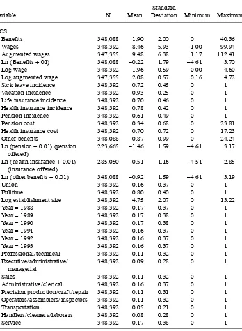
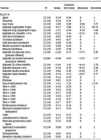
We restrict our sample to private sector workers (jobs in the case of the NCS) whose hourly wages are greater than one dollar and less than 100 dollars in 1982–84 dollars. Descriptive statistics for both the NCS and NLSY79 samples are shown in Table 1. Our NCS sample has 348,392 observations from 7,826 establish-ments over the period 1988–93. Our NLSY79 sample consists of 23,119 observations from 7,178 different individuals over the same period. Note that NLSY79 sample members are ages 22 through 36 during the sample period. Mean log wages and ben-efi t incidence are surprisingly similar between the two samples, although vacation and sick leave are more frequently reported in the NCS. NLSY79 respondents report more professional, managerial, and skilled blue- collar occupations than is indicated in the NCS. (One typically fi nds that the incidence of managerial and professional jobs is higher in household than in establishment surveys; see Abraham and Spletzer 2010).
A. Quits
As discussed above, we fi rst regress ln (B+.01)(hereafter referred to as ln B for sim-plicity) on our control variables using the NCS data, and then use the estimated equa-tion to predict benefi ts for the individuals in the NLSY79 sample. (Using ln(B+.05) instead yields point estimates very close to those in the text.) Our initial NCS regres-sion, which is weighted using the NCS sample weights, has an R2 of 0.861, so the
Table 1
Descriptive Statistics
Variable N Mean
Standard
Deviation Minimum Maximum
NCS
Benefi ts 348,088 1.90 2.00 0 40.36
Wages 348,392 8.46 5.93 1.00 99.94
Augmented wages 347,355 9.48 6.38 1.17 112.41 Ln (Benefi ts +.01) 348,088 –0.22 1.79 –4.61 3.70
Log wage 348,392 1.96 0.59 0.00 4.60
Log augmented wage 347,355 2.08 0.57 0.16 4.72 Sick leave incidence 348,392 0.72 0.45 0 1 Vacation incidence 348,392 0.93 0.25 0 1 Life insurance incidence 348,392 0.70 0.46 0 1 Health insurance incidence 348,392 0.78 0.42 0 1 Pension incidence 348,392 0.61 0.49 0 1
Pension cost 348,392 0.34 0.68 0 23.81
Health insurance cost 348,392 0.70 0.72 0 17.23 Other benefi ts 348,088 0.87 0.99 0 24.24 Ln (pension + 0.01) (pension
offered)
223,665 –1.46 1.59 –4.61 3.17
Ln (health insurance + 0.01) (insurance offered)
285,050 –0.51 1.16 –4.51 2.85
Ln (other benefi ts + 0.01) 348,088 –0.92 1.59 –4.61 3.19
Union 348,392 0.16 0.37 0 1
Fulltime 348,392 0.80 0.40 0 1
Log establishment size 348,392 4.75 2.07 0 13.22
Year = 1988 348,392 0.17 0.37 0 1
Year = 1989 348,392 0.17 0.38 0 1
Year = 1990 348,392 0.17 0.38 0 1
Year = 1991 348,392 0.16 0.37 0 1
Year = 1992 348,392 0.16 0.37 0 1
Year = 1993 348,392 0.16 0.37 0 1
Professional / technical 348,392 0.11 0.32 0 1 Executive / administrative /
managerial
348,392 0.09 0.28 0 1
Sales 348,392 0.11 0.32 0 1
Administrative / clerical 348,392 0.16 0.37 0 1 Precision production / craft / repair 348,392 0.11 0.31 0 1 Operators / assemblers / inspectors 348,392 0.11 0.32 0 1
Transportation 348,392 0.05 0.21 0 1
Handlers / cleaners / laborers 348,392 0.08 0.28 0 1
Service 348,392 0.17 0.38 0 1
Variable N Mean
Standard
Deviation Minimum Maximum
NLSY79
Quits 23,119 0.19 0.39 0 1
Turnover 23,119 0.26 0.44 0 1
Log wage 23,119 1.98 0.49 0.00 4.57
Imputed augmented wages 23,119 9.27 5.06 0.72 98.76 Imputed Log augmented wages 23,119 2.11 0.48 0.16 4.63 Imputed Ln (benefi ts +.01) 23,119 –0.32 1.64 –5.32 3.53 Sick leave incidence 23,119 0.62 0.49 0 1 Vacation incidence 23,119 0.84 0.37 0 1 Life insurance incidence 23,119 0.69 0.46 0 1 Health insurance incidence 23,119 0.80 0.40 0 1
Pension incidence 23,119 0.59 0.49 0 1
Imputed Ln pension costs (pension offered)
13,263 –1.62 0.73 –4.74 2.65
Imputed Ln health insurance (insurance offered)
18,093 –0.66 0.64 –3.51 1.37
Imputed Ln other benefi ts 23,119 –1.04 1.43 –6.44 2.70 Imputed pension costs 23,119 0.29 0.40 –0.42 5.56 Imputed health insurance 23,119 0.66 0.49 –0.50 3.37 Imputed other benefi ts 23,119 0.76 0.72 –0.97 8.71
Union 23,119 0.14 0.35 0 1
Fulltime 23,119 0.92 0.28 0 1
Log establishment size 23,119 4.14 2.25 0 11.51
Year = 1988 23,119 0.16 0.36 0 1
Year = 1989 23,119 0.18 0.38 0 1
Year = 1990 23,119 0.17 0.38 0 1
Year = 1991 23,119 0.16 0.37 0 1
Year = 1992 23,119 0.16 0.37 0 1
Year = 1993 23,119 0.17 0.37 0 1
Professional / technical 23,119 0.14 0.34 0 1 Executive / administrative /
managerial
23,119 0.14 0.35 0 1
Sales 23,119 0.11 0.32 0 1
Administrative / clerical 23,119 0.17 0.38 0 1 Precision production / craft /
repair
23,119 0.15 0.35 0 1
Operators / assemblers / inspectors
23,119 0.09 0.29 0 1
Transportation 23,119 0.05 0.21 0 1
Handlers / cleaners / laborers 23,119 0.05 0.21 0 1
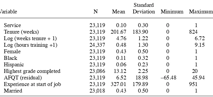
Table 1 (continued)
Table 1 (continued)
Variable N Mean
Standard
Deviation Minimum Maximum
Service 23,119 0.10 0.30 0 1
Tenure (weeks) 23,119 201.67 183.90 0 824 Log (weeks tenure + 1) 23,119 4.76 1.22 0 6.72 Log (hours training +1) 24,337 0.48 1.30 0 9.15
Female 23,119 0.43 0.50 0 1
Black 23,119 0.11 0.32 0 1
Hispanic 23,119 0.06 0.23 0 1
Highest grade completed 23,086 13.12 2.25 0 20 AFQT (residual) 23,119 6.52 18.98 –65.48 45.94 Experience at start of job 23,119 327.01 179.89 0 951
Married 23,018 0.43 0.50 0 1
Our results for quits using the NLSY79 data are shown in Table 2. For comparison purposes, and to verify that the presence of fringe benefi ts actually reduces quits, we fi rst estimate a specifi cation using ln W (not augmented by mandatory benefi ts) and dummies for the incidence of the fi ve benefi ts in the NLSY79. All of the benefi t coef-fi cients are negative and of substantial size, and three out of fi ve are signifi cant at the 5 percent level (using a one- tail test).
The fourth column shows results for a specifi cation using ln B and lnW.9 As the specifi cation is nonlinear the relative magnitude of the effects of marginal dollars of B
and W will vary by their specifi c values. We handle this issue in two ways—by calcu-lating effects at specifi c points such as the median, and by estimating the proportion of workers in the sample cohorts for which the effect of a marginal dollar of B is greater in magnitude than the effect of a marginal dollar of W. For both purposes we use the simulated distribution of B rather than the fi tted values.
The coeffi cients on lnW and ln B are approximately equal. As W is always greater than B, and d ln X / dX = 1 / X, the magnitude of the effect of benefi ts on quits is greater than the magnitude of the effect of wages for essentially all points in our sample (or, more precisely, for more than 99.9 percent of the sample on a weighted basis). As shown in the bottom panel of Table 2, at the median values of wages and benefi ts the effect of the marginal dollar of benefi ts is approximately fi ve times that of wages. These fi ndings are consistent with our theoretical model in Section II.
For comparison purposes, in Columns 2 and 3 we show results for specifi cations omitting benefi ts, using ln W in Column 2 and ln W in Column 3. The coeffi cients in both columns are approximately double the estimated wage coeffi cient in Column 4,
The Journal of Human Resources
Table 2
Regression Coeffi cients, Linear Probability Model, Quits (Bootstrap standard errors in parentheses)
Regression Coeffi cients (1) (2) (3) (4) (5) (6) (7)
Ln wages –0.044 –0.051
(0.008) (0.007)
Ln augmented wages –0.057 –0.027 –0.069 –0.073 –0.070
(0.008) (0.009) (0.060) (0.060) (0.039)
Pension offered –0.016
(0.008) Health insurance offered –0.031
(0.013) Life insurance offered –0.011
(0.010)
Sick leave offered –0.029
(0.008)
Vacation offered –0.015
(0.012)
Ln (benefi t costs+0.01) –0.023 –0.028 –0.027 –0.027
(0.003) (0.019) (0.019) (0.014)
Ln benefi ts x Ln wages 0.0045 0.0042 0.0041
Frazis and Loewenstein
983
(Ln benefi ts)2 0.0011 0.0010 0.0011
(0.0024) (0.0024) (0.0021) Employee contributions for health
insurance included in benefi ts? No No No No No No Yes
Demographics included? No No No No No Yes No
R2 0.1021 0.1012 0.0976 0.1012 0.1016 0.1024 0.1016
N 23,119 26,169 23,119 23,119 23,119 22,985 23,119
Effect of wages (or augmented wages) –0.006 –0.007 –0.007 –0.003 –0.003 –0.003 –0.004
at median (0.001) (0.001) (0.001) (0.001) (0.002) (0.002) (0.001)
Effect of benefi ts at median –0.017 –0.013 –0.012 –0.010
(0.002) (0.007) (0.007) (0.005)
Difference in effect at median –0.013 –0.009 –0.010 –0.006
(0.003) (0.008) (0.008) (0.006) Effect of wages (or augmented wages) –0.010 –0.005 –0.007 –0.006 –0.007
at 25th percentile (0.001) (0.002) (0.002) (0.003) (0.002)
Effect of benefi ts at 25th percentile –0.045 –0.041 –0.041 –0.041
(0.006) (0.013) (0.013) (0.010)
Difference in effect at 25th percentile –0.041 –0.035 –0.035 –0.034
showing that one needs to take into account fringe benefi ts when estimating the effect of wages on turnover. Moreover, using the dollar cost of fringes reduces the wage coeffi cient by substantially more than using the incidence of specifi c fringes—com-pare Columns 1 and 4.
Next we allow a more general functional form. Specifi cally, Column 5 presents estimates for the quadratic specifi cation given by
(10)
The three quadratic terms are jointly signifi cant at the 10 percent level (p =0.069). As the specifi cation with ln B implies a large marginal effect of small amounts of benefi ts, we also experimented with a specifi cation quadratic in log compensation and ln W , but it did not fi t as well as Equation 10.
The interpretation of the coeffi cients in the quadratic specifi cation is not transparent, but we may note that the estimated effect of the marginal dollar of benefi ts is greater than the effect of the marginal dollar of wages for essentially all (99.7 percent) of the NLSY79 sample.10 However, the p value for the hypothesis that the effect of bene
fi ts is greater than the effect of wages for a majority of the sample is only 0.17.11 At the median values of wages and benefi ts, the marginal dollar of benefi ts reduces quits by 1.3 percentage points, while the marginal dollar of wages reduces quits by 0.3 percent-age points. The 0.9 percentpercent-age point difference is not signifi cant at conventional levels (t = 1.09).
To the extent that reductions in quits from higher benefi ts and wages are proportion-ate to the quit rproportion-ate (and quit rproportion-ates in turn are higher at lower compensation levels), the difference in terms of percentage point reductions will be greater at lower compensa-tion levels and it may be easier to discern the larger effect of benefi ts on quits at lower levels. We fi nd that the estimated difference between the effects of benefi ts and wages is especially large for low values of wages and benefi ts. At the 25th percentile for both wages and benefi ts, a marginal dollar of benefi ts reduces quits at the rate of 4.1 per-centage points while the marginal dollar of wages only reduces quits by 0.7 perper-centage points (the t statistic of the difference is 2.34). As another way of examining differ-ences across the compensation distribution, we divide the sample into halves by simu-lated compensation W +B . In our sample the quit rate is 24.9 percent when imputed compensation Cˆ is less than or equal to the sample median and 12.9 percent when compensation is greater than the median. A marginal dollar of benefi ts has a greater effect on quits for over 99 percent of the observations in each half of the sample. However, while the p value for the half with compensation less than or equal to the median is 0.035, the p value for the half with compensation above the median is 0.265. One obtains almost identical results if instead of using the simulated B one takes pre-dicted compensation to be Cˆ=exp(ln ˆB)+W.
The next to last column in Table 2 shows the effect of adding demographic variables
10. Once again, the stronger effect of benefi ts on quits is due to the dollar cost of benefi ts being less than wages. Indeed, the estimated quit function in Equation 10 is symmetric with respect to W and B if 1w = 1b and 2w = 2b. The data show no evidence against symmetry, as the p value of the relevant chi- square test is 0.81.
11. This p value is computed from the bootstrap distribution of the quadratic coeffi cients. Letting ˆj denote the estimated vector of coeffi cients from bootstrap replication j, j= 1, . . . , 200, for 17 percent of the replica-tions the effect of benefi ts was less for a majority of the sample using ˆj to estimate the effects.
and other personal characteristics. Specifi cally, this regression includes age, highest grade completed, Armed Forces Qualifying Test (AFQT) score,12 labor market experi-ence at the start of the job, and dummies for female, black, Hispanic, and married. The coeffi cients in the table are little changed. Thus, the strong negative relationship between benefi ts and turnover is not due to sorting on characteristics of workers that are observable to us. Of course, we cannot ascertain the importance of sorting on un-observables, but if sorting considerations were truly very important, one might expect the inclusion of demographic variables and an ability proxy to have a larger effect on the benefi ts coeffi cients.
Our NCS data count as benefi t expenditures only employer contributions, not con-tributions by employees from wages even though such concon-tributions might be man-datory. Employees may have wages deducted from their paycheck to pay for health insurance or retirement benefi ts. Mandatory deductions for defi ned benefi t pensions are relatively rare in the private sector in the period covered by our data—for example, only 3 percent of defi ned benefi t plans in medium and large private establishments required an employee contribution in 1993 (Bureau of Labor Statistics 1994). Further-more, voluntary deductions for defi ned contribution plans have close substitutes in the form of Individual Retirement Accounts, so the distinction between these contribu-tions and wages is not clear. However, employees cannot typically easily purchase health insurance at rates comparable to those that fi rms can purchase, so employee contributions for health insurance arguably should be classifi ed as benefi ts and not wages.
Accordingly, we estimate an alternative specifi cation in which estimated employee contributions for health insurance are deducted from wages and added to benefi ts. The NCS does not have information on employee contributions for health insurance for all of the years of our analysis. However, it does contain partial information on such con-tributions for the years 1993 and 1994. We use these data to impute the percentage of health benefi ts paid by the fi rm, so that total health expenditures are Hˆ =H/ ˆP , where
H is the cost to the employer of providing health insurance as recorded in the NCS data and Pˆ is the imputed proportion of total contributions paid for by the employer. The predicted value of total health insurance contributions is substituted for H in add-ing up total benefi ts, and the estimated employee contribution is subtracted from wages. Details of the imputation procedure are given in an appendix in our longer working paper.
Results for the quadratic specifi cation are shown in the last column of Table 2. These results are broadly similar to those in the previous specifi cation. The difference at the 25th percentile remains great, although there is some diminution of the effect at the median. The proportion of the NLSY79 sample for which the estimated effect of the marginal dollar of benefi ts is greater than the marginal dollar of wages is reduced to 96.1 percent. For sample respondents with compensation below the median, this proportion is 93.3 percent, but it remains signifi cantly different from 50 percent at the 2 percent level.
One caveat to the above results is that fi rms with higher fringe benefi ts may also have greater nonpecuniary compensation such as more comfortable working condi-tions. Such nonpecuniary compensation, which can be thought of as unobserved fringe
benefi ts, would imply that our estimates exaggerate the effect of benefi ts on turnover. However, note that we estimate the effect of each dollar of wages and benefi ts to be roughly equal, with the larger marginal effect of benefi ts occurring because the effects are nonlinear and benefi t costs are much lower than wages. In order to explain the larger mar-ginal effect of benefi ts, unobservable nonpecuniary compensation would have to be of a suffi cient magnitude to bring benefi ts and wages into rough equality, which is implausible.
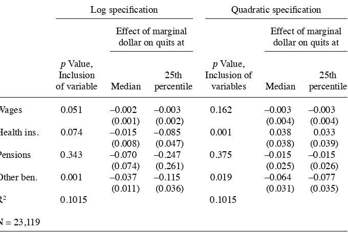
Finally, we attempt to estimate the effects of individual benefi ts. To simplify our task somewhat and to focus on the most widely researched benefi ts, we aggregate va-cations, sick leave, life insurance, and the benefi ts with incidence not collected in the NLSY79 into a single “other” category, thus estimating the effects for the three bene-fi ts: pensions, health insurance, and “other.” Log pension and health costs are imputed as Iiln Bpi , where Ii is an indicator for benefi t i (i = [pension, health insurance]) and lnpBi is the imputed value of the log of benefi t i using the coeffi cients from a regression estimated with NCS observations where benefi t i is present. The R2 for the regression for log pension costs (log health insurance costs) where pensions (health insurance) are offered is 0.308 (0.381). The R2 for the log of other bene
fi ts is 0.813.
We fi rst discuss results from a specifi cation linear in log benefi ts. (The p value of the additional terms in a quadratic- in- logs specifi cation is 0.168.) Standard errors are derived from 100 bootstrap replications. In this specifi cation, shown in the left side of Table 3, the coeffi cients on wages and health insurance are signifi cantly different from zero at the 10 percent level and other benefi ts are signifi cant at the 1 percent level. Signifi cance levels are similar for the difference between the effect of a marginal
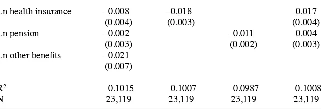
dol-Table 3
Effects of Individual Benefi ts on Quits, Log and Quadratic Specifi cations
Log specifi cation Quadratic specifi cation
Effect of marginal dollar on quits at
Effect of marginal dollar on quits at
p Value, Inclusion
of variable Median
25th percentile
p Value, Inclusion of
variables Median
25th percentile
Wages 0.051 –0.002 –0.003 0.162 –0.003 –0.003 (0.001) (0.002) (0.004) (0.004) Health ins. 0.074 –0.015 –0.085 0.001 0.038 0.033
(0.008) (0.047) (0.038) (0.039) Pensions 0.343 –0.070 –0.247 0.375 –0.015 –0.015
(0.074) (0.261) (0.025) (0.026) Other ben. 0.001 –0.037 –0.115 0.019 –0.064 –0.077
(0.011) (0.036) (0.031) (0.035)
R2 0.1015 0.1015
lar of wages and a marginal dollar of these two benefi ts. The pension coeffi cient is not signifi cantly different from zero. Not surprisingly, standard errors are for the most part larger than in specifi cations aggregating benefi ts, and given the large standard error on the marginal dollar of pensions—0.074 at the median—it would be surprising if the effect was large enough to be signifi cant at conventional levels.
A specifi cation quadratic in benefi ts is shown on the righthand side of Table 3. The fi t is similar for the two specifi cations. However, the effect of the marginal dollar of health insurance is now substantially wrong- signed, though not signifi cant. The differ-ence between the effect of the marginal dollar of wages and other benefi ts is signifi cant at the 10 percent level at the median and at the 5 percent level at the 25th percentile. The equivalent differences for pensions and health insurance are not signifi cant.
Our overall conclusion is that the estimates for the effects of individual benefi ts are imprecise and volatile. Part of the reason for this is that the incidences of the individual benefi ts are strongly correlated with each other and with wages. This is demonstrated in the fi rst panel of Table 4, which shows the correlation matrix for ln W and the indi-vidual benefi t incidences in the NLSY79. Benefi t cost is even more highly correlated across benefi ts, as shown in the bottom panel of Table 4. The higher correlation of cost relative to incidence is due to the association of the incidence of individual benefi ts with higher costs for other benefi ts. An appendix to our longer working paper shows the coeffi cients on cross- benefi t incidence dummies (and log wages) from our NCS
Table 4
Wage and Benefi t Correlations, NLSY79
Correlations, Log Wage and Benefi t Incidence
Ln Wage
Life Insurance offered 0.30 0.58 0.69 0.48 1
Sick leave offered 0.25 0.36 0.43 0.49 0.40 1
Correlations, Log Augmented Wages and Imputed Log Benefi t Costs
regressions on individual benefi ts. These coeffi cients are generally positive and often of substantial magnitude. The combined effect of the positive association of the incidence of individual benefi ts with both the incidence and cost of other benefi ts is to make it dif-fi cult to disentangle the effects of different benefi ts upon quits. Note that these positive associations are consistent with our theory. If all types of benefi ts had a greater effect on quits than wages, fi rms especially concerned with reducing quits would be expected to offer several types of benefi ts and to more generously fund those they did offer.
The large correlations between benefi ts also imply that examining the effect of ben-efi ts individually may greatly exaggerate their effect on quits. Table 5 shows examples of this with specifi cations using logs of (augmented) wages and individual benefi ts (without quadratic terms). Entered separately, both health insurance and pensions have large and signifi cant effects on quits. Entered together but without other benefi ts, the effect of pensions is cut by almost three- quarters and is no longer signifi cant; the effect of health insurance drops slightly. Entered with other benefi ts, the effect of pensions drops further and the effect of health insurance is cut by more than half. Papers dealing with the effect of individual benefi ts on turnover should be read with this in mind.13
B. Turnover
Table 6 shows the results with turnover rather than quits as the dependent variable. For aggregate benefi ts, the results are similar to but stronger than the results for quits. Again, there is no evidence against symmetrical wage and benefi t effects. Note that the difference between the estimated effects of wages and benefi ts is larger than for quits at various points in the compensation distribution, with a difference of 8.2 percentage points at the 25th percentile and 3.0 percentage points for the median (both are signifi -cant at the 1 percent level). Specifi cations using health, pensions, and “other” benefi ts show results that are similarly volatile and imprecise to those for quits.
13. As noted above, papers analyzing turnover typically analyze the effect of only one individual benefi t. Mitchell (1983) has the most comprehensive information on fringes. Unlike us, Mitchell fi nds that including other fringes has only a small effect on the pension coeffi cient in a quit or turnover equation.
Table 5
Regression Coeffi cients for Health Insurance and Pension Costs, Quit Regression
Ln health insurance –0.008 –0.018 –0.017
(0.004) (0.003) (0.004)
Ln pension –0.002 –0.011 –0.004
(0.003) (0.002) (0.003)
Ln other benefi ts –0.021 (0.007)
R2 0.1015 0.1007 0.0987 0.1008
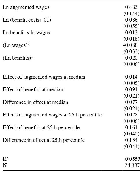
C. Training
Our model predicts that fi rms that pay a higher proportion of compensation in the form of benefi ts will predominantly be fi rms with greater hiring and training costs. One obvious proxy for training costs is the amount of formal training provided to the employee, which the NLSY79 provides data on. We regressed the log of hours (plus one) of formal training with the current employer in the previous year on wages and benefi ts, using the same quadratic specifi cation as in Equation 10 (with the exception that we use a cubic in tenure rather than log tenure on the basis of fi t). The results, shown in Table 7, support our model. Both wages and benefi ts are signifi cantly as-sociated with training, but in the range of most of the data the effect of benefi ts is much larger. At the median, a dollar increase in benefi ts is associated with six times the increase in log training that a dollar increase in wages is. Similarly, we fi nd that for 86.6 percent of the sample the marginal effect of benefi ts exceeds that of wages (with a standard error of 4.3 percent).
V. Conclusion
It has been argued that one of the functions of fringe benefi ts is to re-duce turnover. We have investigated this question both theoretically and empirically. Our theoretical model shows how it is possible in a competitive equilibrium that the marginal dollar of benefi ts would reduce quits more than the marginal dollar of wages.
For our empirical work, we turned to an untapped data source, the National Com-pensation Survey, to analyze the responsiveness of quits to fringe benefi ts. Specifi -cally, by combining information in the NCS on the cost of benefi ts with information on worker quits and fringe benefi t incidence in the NLSY79, we have been able to estimate the quit probability as a function of a worker’s wage and the dollar value of his fringe benefi ts.
While our estimation procedure is reduced- form and thus sheds light on causal-ity only indirectly, our results are consistent with employers using fringe benefi ts to reduce quits. Our estimates indicate that an additional dollar of fringe benefi ts is more strongly associated with lower quits than is an additional dollar of wages. Consistent with our theoretical model, which predicts a positive association between benefi ts and turnover costs, we fi nd that employers who provide more training and presumably have greater turnover costs offer greater benefi ts.
The Journal of Human Resources
Table 6
Regression Coeffi cients, Linear Probability Model, Turnover (Bootstrap standard errors in parentheses)
(1) (2) (3) (4) (5) (6) (7)
Regression coeffi cients
Ln wages –0.051 –0.063
(0.009) (0.008)
Ln augmented wages –0.071 –0.023 –0.015 0.011 –0.057
(0.009) (0.010) (0.067) (0.067) (0.043)
Pension offered –0.032
(0.009) Health insurance offered –0.042
(0.014) Life insurance offered –0.019
(0.011) Sick leave offered –0.031
(0.009)
Vacation offered –0.043
(0.013)
Ln (benefi t costs+.01) –0.037 –0.066 –0.060 –0.052
(0.004) (0.021) (0.022) (0.016)
Ln benefi ts x ln wages 0.0111 0.0098 0.0066
(0.0073) (0.0073) (0.0055)
(Ln wages)2 0.0006 –0.0008 0.0076
Frazis and Loewenstein
991
Employee contributions for health
insurance included in benefi ts? No No No No No No Yes
Demographics included? No No No No No Yes No
R2 0.1579 0.1559 0.1492 0.1565 0.1568 0.1606 0.1566
N 23,119 26,169 23,119 23,119 23,119 22,985 23,119
Marginal Effects
Effect of wages (or augmented –0.007 –0.009 –0.009 –0.003 –0.001 0.001 –0.003 wages) at median (0.001) (0.001) (0.001) (0.001) (0.002) (0.002) (0.001)
Effect of benefi ts at median –0.027 –0.031 –0.029 –0.022
(0.003) (0.007) (0.008) (0.006)
Difference in effect at median –0.024 –0.030 –0.030 –0.019
(0.004) (0.009) (0.009) (0.007)
Effect of wages (or augmented –0.012 –0.004 –0.003 0.000 –0.006
wages) at 25th percentile (0.001) (0.002) (0.003) (0.003) (0.002)
Effect of Benefi ts at 25th –0.073 –0.085 –0.078 –0.075
percentile (0.008) (0.015) (0.015) (0.011)
Difference in effect at 25th –0.069 –0.082 –0.079 –0.069
Appendix 1
Signing the Imputation Bias
from the Omission of Tenure
In this appendix we evaluate the bias resulting from the imputation of benefi ts given that tenure is included in the quit regressions but not the imputation procedure. We show that if tenure and the benefi t incidence dummies all have positive coeffi cients in a regression of benefi ts on the covariates observed in the NCS plus ten-ure, we will underestimate the effect of benefi t expenditure on quits relative to wages.
We take as an example the specifi cation in the fourth column of Table 2:
(A1) Q=βwlnW+βblnB+X
X+βTlnT+e
Table 7
Regression Coeffi cients, Log (Training Hours + 1), Current Employer in Previous Year
Ln augmented wages 0.483
(0.144) Ln (benefi t costs+.01) 0.086
(0.055) Ln benefi t x ln wages 0.013
(0.018)
(Ln wages)2 –0.088
(0.033)
(Ln benefi ts)2 0.020
(0.006)
Effect of augmented wages at median 0.014 (0.005) Effect of benefi ts at median 0.091
(0.021) Difference in effect at median 0.077
(0.024) Effect of augmented wages at 25th percentile 0.028
(0.006) Effect of benefi ts at 25th percentile 0.161
(0.040) Difference in effect at 25th percentile 0.134
(0.044)
R2 0.0553
where T denotes tenure and e is a residual orthogonal to the covariates. Substituting imputed benefi ts for the unobserved actual benefi ts (and ignoring the difference be-tween imputed and actual W , as in the text), Equation A1 becomes:
(A1’) Q=βwlnW+βblnpB+X
X+βTlnT+[βb(lnB−lnpB)+e],
where the term in brackets is the residual of the equation as estimated.
To evaluate the bias stemming from estimating Equation A1’ instead of Equation A1, consider U ≡lnB−lnpB as an omitted variable and apply the formula for omitted- variable bias:
(A2) bw=βw+βbδw
bb=βb+βbδb
where bw and bb denote the estimated coeffi cients on lnW and lnpB in Equation A1’ and where δw, δb, and δT denote the coeffi cients on lnW, lnpB, and ln T in a regression of U
on [lnW, lnpB,X, lnT]. (Here and in what follows, we ignore the distinction between sample and population for convenience.)
Claim 1: Let χ ≡ βb/B− βw/W denote the difference between the estimated ef-fect of a marginal dollar of benefi ts and a marginal dollar of wages on quits at given levels of B and W were one able to estimate Equation A1 using actual benefi ts and let D≡bb/B−bw/W denote the difference between the estimated effects of benefi ts and wages when one estimates Equation A1’ using predicted benefi ts. Then
(A3) bw− βw=−δTθwbb
(1+δb)
bb− βb=−δTθbbb
(1+δb)
D− χ=−δTbb
1+δb( θb
B −
θw W ) ,
where θb and θw denote the coeffi cients on lnpB and lnW in a regression of ln T
on [lnW, lnpB,X].
Proof: The system A2 can be simplifi ed as follows. Note that lnpB is constructed as a predicted value from a regression on X, ln W, and benefi t incidence dummies. Consider the regression
(A4) U=dwlnW +dblnpB+Xd x+η .
Since OLS prediction errors are uncorrelated with regressors, the coeffi cients dw, db, and dx are all zero. The w and b coeffi cients in Equation A2 are related to the dw
and db coeffi cients through the omitted- variable bias formula: (A5) dw=δw+δTθw=0
From Equation A5, it follows that w = − Tθw and b = − Tθb . Substituting these results into Equation A2 and rearranging, we obtain Equation A3. Q.E.D.
To determine the bias in bw, bb, and D, we must sign T and − T / (1 – b). Let V
denote the vector of control variables in the predicted benefi ts equation that are not in-cluded in the quit Equation A1 (that is, the vector Z in the paper is given by Z = [X V]). Specifi cally, in our empirical work, V consists of the benefi t incidence variables. As a fi rst step, write predicted benefi ts as a least squares projection on V, W, and X:
(A6) lnpB=V(␣
V+αT␥V)+(αW+αTγW) lnW +X(␣X+αT␥X),
where αT is the coeffi cient that we would see on ln T were it also included in Equation A6 and where ␥V, w, and ␥X denote the coeffi cients on V, lnW, and Xin a regression of ln T on [V, lnW, X].
To simplify the ensuing analysis, let V* and ln T*, respectively, denote the residuals from regressions of V and ln T on lnW and X. From the discussion in Goldberger (1991, pp. 185–86), we know that that the residual of the regression of lnpB on lnW and X is given by lnpB*=V *(␣V+αT␥V). Also, denoting the least squares projection of U on lnpB* and ln T* as
(A7) U=δb*lnpB*+δT*lnT*,
we know that δb*=δb and δT*=δT.
We now relate b* and T* to the parameters in Equation A6. Claim 2: Let ε ≡lnT*−V*␥
V denote the residual from a regression of ln T* on
V* and let λ denote the coeffi cient on lnpB* from a simple regression of ln T* on lnpB* . Then
(A8) δb*=D
1D2, where
D1≡ −Var(ε)
Var(lnT*)− λCov(lnpB*, lnT*) ,
D2≡ (␣V+αT␥V)V*'V*(αT␥V) (␣V+αT␥V)V*'V*(␣V+αT␥V)
.
Proof: The coeffi cient b1 of a variable X1 from a regression of Y on two variables
X1, X2, and a constant is given by b
1=
Cov(X1,Y) Var(X2)−Cov(Y,X2) Cov(X1,X2)
Var(X
1) Var(X2)−Cov(X1,X2) 2
(for instance, see Gujarati 1978, p. 103). Correspondingly, the estimated coeffi -cient on lnpB* in (A7) is given by
(A9) δb*= Cov(lnpB*,U) Var(lnT*)−Cov(U, lnT*) Cov(lnpB*, lnT*) Var(lnpB*) Var(lnT*)−Cov(lnpB*, lnT*)2