Comprehensive data warehouse exploration with qualified
association-rule mining
Nenad Jukic´
a,*, Svetlozar Nestorov
b,1a
School of Business Administration, Loyola University Chicago, 820 N. Michigan Avenue, Chicago, IL 60640, USA
b
Department of Computer Science, The University of Chicago, Chicago, IL, USA
Received 10 May 2004; received in revised form 9 July 2005; accepted 11 July 2005 Available online 11 August 2005
Abstract
Data warehouses store data that explicitly and implicitly reflect customer patterns and trends, financial and business practices, strategies, know-how, and other valuable managerial information. In this paper, we suggest a novel way of acquiring more knowledge from corporate data warehouses. Association-rule mining, which captures co-occurrence patterns within data, has attracted considerable efforts from data warehousing researchers and practitioners alike. In this paper, we present a new data-mining method called qualified association rules. Qualified association rules capture correlations across the entire data warehouse, not just over an extracted and transformed portion of the data that is required when a standard data-mining tool is used.
D2005 Elsevier B.V. All rights reserved.
Keywords:Data warehouse; Data mining; Association rules; Dimensional model; Database systems; Knowledge discovery
1. Introduction
Data mining is defined as a process whose objec-tive is to identify valid, novel, potentially useful and understandable correlations and patterns in existing data, using a broad spectrum of formalisms and tech-niques[9,23]. Mining transactional (operational)
data-bases, containing data related to current day-to-day organizational activities could be of limited use in certain situations. However, the most appropriate and fertile source of data for meaningful and effective data mining is the corporate data warehouse, which contains all the information from the operational data sources that has analytical value. This information is integrated from multiple operational (and external) sources, it usually reflects substantially longer history than the data in operational sources, and it is struc-tured specifically for analytical purposes.
The data stored in the data warehouse captures many different aspects of the business process across
0167-9236/$ - see front matterD2005 Elsevier B.V. All rights reserved.
doi:10.1016/j.dss.2005.07.009
* Corresponding author. Tel.: +1 312 915 6662. E-mail addresses:[email protected]
(N. Jukic´), [email protected] (S. Nestorov). 1Tel.: +1 773 702 3497.
various functional areas such as manufacturing, dis-tribution, sales, and marketing. This data explicitly and implicitly reflects customer patterns and trends, business practices, organizational strategies, financial conditions, know-how, and other knowledge of poten-tially great value to the organization.
Unfortunately, many organizations often underuti-lize their already constructed data warehouses[12,13]. While some information and facts can be gleaned from the data warehouse directly, through the utiliza-tion of standard on-line analytical processing (OLAP), much more remains hidden as implicit patterns and trends. The standard OLAP tools have been perform-ing well their primary reportperform-ing function where the criteria for aggregating and presenting data are speci-fied explicitly and ahead of time. However, it is the discovery of information based on implicit and pre-viously unknown patterns that often yields important insights into the business and its customers, and may lead to unlocking hidden potential of already collected information. Such discoveries require utilization of data mining methods.
One of the most important and successful data mining methods for finding new patterns and correla-tions is association-rule mining. Typically, if an orga-nization wants to employ association-rule mining on their data warehouse data, it has to use a separate data-mining tool. Before the analysis is to be performed, the data must be retrieved from the database reposi-tory that stores the data warehouse, transformed to fit the requirements of the data-mining tool, and then stored into a separate repository. This is often a cum-bersome and time-consuming process. In this paper we describe a direct approach to association-rule data mining within data warehouses that utilizes the query processing power of the data warehouse itself without using a separate data mining tool.
In addition, our new approach is designed to answer a variety of questions based on the entire set of data stored in the data warehouse, in contrast to the regular association-rule methods which are more suited for mining selected portions of the data warehouse. As we will show, the answers facilitated by our approach have a potential to greatly improve the insight and the actionability of the discovered knowledge.
This paper is organized as follows: in Section 2 we describe the concept of association-rule data mining and give an overview of the current limitations of
association-rule data mining practices for data ware-houses. Section 3is the focal point of the paper. In it we first introduce and define the concept of qualified association rules. In 3.1 we discuss how qualified association rules broaden the scope and actionability of the discovered knowledge. In3.2we describe why existing methods cannot be feasibly used to find qualified association rules. In 3.3 3.4 and 3.5 we offer details of our own method for finding qualified association rules. In Section 4 we describe an illus-trative experimental performance study of mining real world data that uses the new method we introduced. And finally, inSection 5we offer conclusions.
2. Association-rule data mining in data warehouses
The standard association-rule mining [1,2] dis-covers correlations among items within transactions. The prototypical example of utilizing association-rule mining is determining what products are found together in a basket at a checkout line at the super-market; hence the often-used term: market basket analysis [4]. The correlations are expressed in the following form:
Transactions that contain X are likely to contain Y
as well noted asXYY, whereXand Yrepresent sets
of transaction items. There are two important quanti-ties measured for every association rule:support and
confidence. The support is the fraction of transactions
that contain bothXandYitems. The confidence is the fraction of transactions containing itemsX, which also contain itemsY. Intuitively, the support measures the significance of the rule, so we are interested in rules with relatively high support. The confidence measures the strength of the correlation, so rules with low confidence are not meaningful, even if their support is high. A rule in this context is the relationship among transaction items with enough support and confidence.
The standard association rule mining process employs the basic a-priori algorithm[1,3]for finding sets of items with high support (often calledfrequent
itemsets). The crux of the a-priori approach is the
that need to be counted, starting by eliminating single items that are infrequent. For example, if we are looking for all sets of items (pairs, triples, etc. . .)
that appear together in at least s transactions, we can start by finding those items that by themselves appear in at leaststransactions. All items that do not appear on their own in at least s transactions are pruned out.
In practice, the discovery of association rules has two phases. In the first phase, all frequent itemsets are discovered using the a-priori algorithm. In the second phase, the association rules among the frequent item-sets with high confidence are constructed. Since the computational cost of the first phase dominates the total computational cost[1], association-rule mining is often defined as the following question pertaining to transactional data, where each transaction contains a set of items:
What items appear frequently together in transactions?
Association-rule data mining has drawn a consid-erable amount of attention from researchers in the last decade. Much of the new work focuses on expanding the extent of association-rule mining, such as mining generalized rules (i.e. when transaction items belong to certain types or groups, generalized rules find associations among such types or groups) [14,24]; mining correlations and casual structures, which finds generalized rules based on implicit correlations among items, while taking into consideration both the presence and the absence of an item in a transaction
[6,22]; finding association rules for numeric attributes, where association rules, in addition to Boolean con-ditions (i.e. item present in the transactions), may consider a numeric condition (e.g. an item that has a numeric value, must have a value within a certain range) [10,11]; finding associations among items occurring in separate transactions[17,19,27]; etc.
In this paper we introduce qualified association
rulesas a way of extending the scope of association
rule mining. Our method extends the scope of asso-ciation rule mining to include multiple database rela-tions (tables), in a way that was not previously feasible. This approach is designed to provide a real addition to the value of collected organizational infor-mation and is applicable in a host of real world situations, as we will illustrate throughout this paper. Many of the previously proposed association-rule extensions are either applicable to a relatively narrow
set of problems, or represent a purely theoretical advance. In addition, they also often require computa-tional resources that may be unrealistic for most of the potential organizational users. In contrast, our pro-posed method is both broadly applicable and highly practical from the implementation and utilization points of view.
Dimensional modeling [16], which is the most prevalent technique for modeling data warehouses, organizes tables into fact tables, containing basic quantitative measurements of an organizational acti-vity under consideration, and dimension tables that provide descriptions of the facts being stored. Dimen-sion tables and their attributes are chosen for their ability to contribute to the analysis of the facts being stored in the fact tables.
The data model that is produced by the dimen-sional modeling method is known as a star-schema
[7] (or a star-schema extension such as snowflake or constellation). Fig. 1 shows a simple star-schema model of a data warehouse for a retail company. The fact table contains the sale figures for each sale transaction and the foreign keys that connect it to the four dimensions: Product, Customer, Location, and Calendar.
Consider the data warehouse depicted by Fig. 1. The standard association-rule mining question for this environment would be:
What products are frequently bought together?
This question examines the fact table as it relates to the product dimension only. A typical data warehouse, however, has multiple dimensions, which are ignored
LOCATION
by the above single-dimension question, as illustrated byFig. 2.
For example, an analyst at the corporate headquar-ters may ask the following question:
What products are frequently bought togetherin a
particular region and during a particular month?
This question requires examination of multiple dimensions of the fact table. Standard association-rule mining approach would not find the answer to this question directly, because it only explores the fact table with its relationship to the dimension table that contains transaction-items (in this case Product), while the other dimension tables (the non-item dimen-sions) are not considered. In fact, by applying stan-dard algorithms directly, we may not discover any association rules in situations when there are several meaningful associations that involve multiple dimen-sions. The following example illustrates an extreme case scenario of this situation.
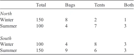
Example 1. A major retail chain operates stores in two regions: South and North; and divides the year into two seasons: Winter and Summer. The retail chain sells hundreds of different products including sleeping bags and tents.Table 1shows the number of transactions for each region in each season as well as the percentage of transactions that involved a sleeping bag, a tent, or both.
Suppose we are looking for association rules with 0.5% support and 50% confidence. Let’s first consider the transactions in all regions and all seasons. There are 500 thousand transactions and only 10 thousand of them involve both a sleeping bag and a tent, so the
support of the pair of items is 2% (greater than 0.5%). There are 25 thousand transactions that involve sleep-ing bags, 23 thousand transactions that involve tents. Therefore the confidence of sleeping bag Y tent is 40% and the confidence of tent Y sleeping bag is 43%. Thus, no association rule involving sleeping bags and tents will be discovered. Let’s consider the transactions in the North region separately. In the North sleeping bags appear in 12 thousand transac-tions, tents appear in 9 thousand transactransac-tions, and both sleeping bags and tents appear together in 4 thousand transactions. The support2for both items is 0.8% (greater than 0.5%) but the confidence for rules involving sleeping bag and tent are 33% and 44% (both less than 50%). Thus, no association rule invol-ving bags and tents will be discovered. Similarly, no rules involving both sleeping bag and tent will be discovered in the South, and no associations will be discovered between sleeping bags and tents when we consider all the transactions in each season (Summer and Winter) separately.
These conclusions (no association rules) are rather surprising becauseif each combination of region and
season were considered separately the following
association rules would be discovered:
nsleeping bagYtent; in the North during the Sum-mer (sup = 0.60%, conf = 75%)
nsleeping bagYtent; in the South during the Winter (sup = 0.60%, conf = 75%)
ntentYsleeping bag; in the South during the Sum-mer (sup = 0.60%, conf = 50%)
Fig. 2. Association-rule data mining scope for the example retail company star schema.
Table 1
Transaction statistics (in thousands) for Example 1
Total Bags Tents Both
Standard association rule mining cannot discover these association rules directly, because it does not account for non-item dimensions.
In addition to the possibility of suppressing some of the existing relevant rules (as illustrated by Exam-ple 1), another type of problem can arise when multi-ple dimensions are not considered: an overabundance of discovered rules may hide a smaller number of meaningful rules. Example 2 illustrates an extreme case scenario of this situation.
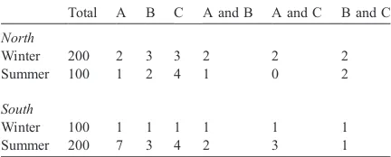
Example 2.Another major retail chain also operates stores in two regions: South and North; and divides the year into two seasons: Winter and Summer. This retail chain sells hundreds of different products including Product A, Product B, and Product C.
Table 2 shows the number of transactions for each region in each season; the number of transactions that involved Product A, Product B, Product C; as well as the number of transactions that involved Product A and Product B together, Product A and Product C together, and Product B and Product C together.
Suppose we are looking for association rules with 0.50% support and 50% confidence. If we consider the transactions in all regions and all seasons we will discover that every possible association rule invol-ving two items satisfies the threshold, as shown below:
nProduct A Y Product B (sup = 1.00%, conf = 55%)
nProduct B Y Product A (sup = 1.00%, conf = 67%)
nProduct A Y Product C (sup = 1.00%, conf = 55%)
nProduct C Y Product A (sup = 1.00%, conf = 50%)
nProduct B Y Product C (sup = 1.00%, conf = 67%)
nProduct C Y Product B (sup = 1.00%, conf = 50%).
In this example, any combination of two of the three products is correlated. Thus, it is difficult to make any conclusions, reach any decisions, and take any actions. This problem occurs when a mining process produces a very large number of rules, thus proving to be of little value to the user. However if we consider each region and season separately we will find only one rule within the given support and con-fidence limit:
nProduct CYProduct A; in the South during the Summer (sup3= 0.50%, conf = 75%).
Isolating this rule may provide valuable additional information to the user. The above two examples illustrate two types of situations in which association rules that consider both item-related dimension (e.g. Product) and non-item related dimensions (e.g. Region, Session) add new insight into the nature of data to the user. Section 3 describes the method that enables such discoveries.
2.1. Related work
Recent work on mining the data warehouse has explored several approaches from different perspec-tives. Here we give a brief overview.
Both Refs. [15,21] extend OLAP techniques by finding patterns in the form of summaries or trends among certain cells of the data cube. While both papers examine multiple dimensions of the data ware-house, neither discovers correlations among multiple values of the same dimension. For example, the tech-niques detailed in Ref. [15] can discover that bthe average number of sales for all camping products combined (tents and bags) is the same during the Winter in the South and during the Summer in the North.Q However, their framework does not handle association rules involving multiple products bought in the same transactions, e.g.bnumber of transactions Table 2
Transaction statistics (in thousands) for Example 2
Total A B C A and B A and C B and C
North
Winter 200 2 3 3 2 2 2
Summer 100 1 2 4 1 0 2
South
Winter 100 1 1 1 1 1 1
Summer 200 7 3 4 2 3 1
involving both tents and bags is the same during the Summer in the North and for all seasons in the SouthQ. The framework presented in Ref.[21]can find sum-marized rules associated with a single item. For exam-ple, it can reduce the fact thatbduring the Winter the number of tents sold in the South is equal or greater than the number sold in the NorthQ to the rule that
bduring the Winter the number of sales for all cam-ping products in the South is equal or greater than the number of sales in the NorthQ, if such a reduction holds. However, rules about multiple products sold in the same transaction lie beyond this framework.
The focus of Ref.[25] is on finding partitions of attribute values that result in interesting correlations. In contrast to our work, quantitative rules involve at most one value or one value range for each attribute. For example, btransactions involving a tent in the North are likely to occur during the SummerQ is a quantified rule, whereas btransactions involving a tent in the North are likely to involve a bagQ is a qualified rule that falls outside of the scope of quan-tified rules because it involves two values of the Product dimension.
Generalized association rules [24] and multiple-level association rules [8] capture correlations among attribute values, possibly at different levels, within the same dimensional hierarchy but not across multiple dimensions. For example, btransactions involving sporting goods tend to involve sunscreenQ
is within the framework of generalized rules and multi-level rules, while the qualified rulebtransaction involving sporting goods tend to involve sunscreen in the summerQis beyond their scope.
A precursor to qualified association rules is dis-cussed in Ref. [18] with the focus on dealing with aggregate rather than transactional data.
3. Qualified association rules
Standard association rules express correlations between values of a single dimension of the star schema. However, as illustrated by Examples 1 and 2, values of the other dimensions may also hold important correlations. For example, some associa-tions become evident only when multiple dimensions are involved. In Example 1, sleeping bags and tents appear uncorrelated in the sales data as a whole, or
even when the data is considered separately by region or season. Yet, several association rules are discovered if the focus is on the data for a particular region during a particular season. One such rule isbsleeping bagY tentQ for the transactions that occurred in the North region during the Summer season. This association rule involves more than just a pair of products; it also involves the location as well as the time period of the transaction. In order to capture this additional infor-mation, we can augment the association rule notation as illustrated by the following qualified association rule:
sleeping bagYtent½region¼North; season¼Summer:
We define qualified association rule as follows: LetTbe a data warehouse whereX andYare sets of values of the item-dimension. Let Q be a set of equalities assigning values to attributes of other (non-item) dimensions ofT. Then,XYY[Q] is a qualified association rule with the following interpretation: Transactions that satisfy Q and contain X are likely to contain Y.
For a more detailed definition consider a star schema with d dimensions. Let the fact table be F
and the dimensions be D0. . .Dd. The schema of
dimension table Di consists of a key ki and other
attributes. The schema of the fact table F contains the keys for all dimensions,k0. . .kd, and a transaction
id attributetid.
Without loss of generality, we can assume that the item dimension is D0, so the set of all items is
domain(k0). For all other dimensionsDjwe can assert
that the functional dependencytidYkjholds forF(i.e. each value oftidin the fact table determines one and only one vale ofkjin the non-item dimension tableDj).
We define aqualifierto be a set of equalities of the form:attr=value whereattris a non-key attribute of any of the non-item dimensions and value is a con-stant. For example, {region=North} is a qualifier and so is {season = Summer; region = South}.
We define a valid qualifier to be a qualifier that contains at most one equality for each non-item dimension. Examples of valid qualifiers are {
sea-son = Summer; region = South} and {region = South;
gender = Male}; while examples of invalid qualifiers
are: {region = North; region = South} and {season =
con-sider valid qualifiers, and for brevity, refer to them as qualifiers.
Now, we define a qualified association rule:
XYY Q½
where X and Y are itemsets (X odomain(k0); Y o
domain(k0)) andQis a qualifier. For example,
sleeping bagYtent½region¼North; season¼Summer
is a qualified association rule. The intuitive interpreta-tion of this rule is that if a transacinterpreta-tion includes a sleep-ing bag in the North region dursleep-ing the Summer season, then the transaction is likely to also include a tent. Before defining the support and confidence of a qualified association rule, we need to define the sup-port of a qualified itemset. LetIbe an itemset andQa qualifier. Then,I[Q]is a qualified itemset. For exam-ple, {sleeping bag, tent} [region = North, season =
Summer] is a qualified itemset. The s_count of a
qualified itemset I[Q], denoted as s_count(I[Q]), is the number of transactions that contain the itemset and satisfy all equalities inQ.
Formally, support is defined as follows. Let
I= {e1;. . .; em} andQ= {a1=v1;. . .; ap=vp}. Without
loss of generality we can assume thataiis an attribute
ofDi. Then,s_count(I[Q]) is equal to the size of the
following set:
S¼
tjafiaF;i¼1::m;djaDj;j¼1::p;fi½tid
¼t;fi½ ¼k0 ei;fikj¼djkj;dj a j¼vjg:
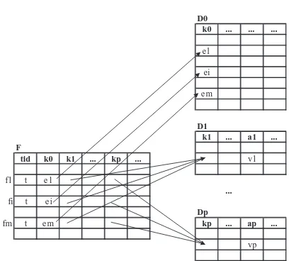
The setSconsists of all transaction IDst, for which there aremtuples (i.e. records or table rows) inFthat satisfy the following conditions:
nallm tuples havet as their tid.
nall m tuples agree on all dimension key attributes exceptk0.
nfor every attributekj, its single value in allmtuples
is the value of attribute kj of a tuple in dimension
tableDjwhose value of attribute aj is vj.
These conditions are illustrated inFig. 3.
For example, for the qualified itemset I= {bag, tent}[Q], the set S would consist of all transaction IDs representing transactions that satisfy the qualify-ing conditionQ, for which there are 2 tuples (one for
bag, one for tent) in the fact table that agree on all attributes except for k0(attributek0points tobag for
one tuple and totentfor the other). In other words, set
Swould capture transaction IDs of all transactions: (1) where bag and tent were sold together (2) which satisfy the qualifying condition (e.g. within a particu-lar region and season).
Now, we can define the support and confidence of a qualified association rules as follows:
support Xð YY Q½ Þ ¼ s count Xðð [YÞ½ QÞ
s countðF F½ Þ
confidence Xð YY Q½ Þ ¼s count Xðð [YÞ½ QÞ
s count X Qð ½ Þ
Note that s_count(F[F]) is simply the number of transactions in the fact tableF.
The support and confidence of the rules in G were computed using these definitions.
3.1. Discussion
While qualified association rules are natural exten-sions of standard association rules, they contain more detailed and diverse information which offer several distinct advantages.
First, the phenomenon that brings a qualified rule to existence can be explained more easily. In Example 2, standard association rule mining found the correla-tions between products A, B, and C within the speci-fied confidence and support threshold for all sales.
D0
k0 ... ... ...
e1
ei
e m
D1
k1 ... a1 ...
F
tid k0 k1 ... kp ... v1
f1 t e 1
...
fi t e i
Dp
fm t e m kp ... ap ...
vp
However, only the qualified rule would give the explanation that, once regions and seasons are con-sidered separately, the correlation of sales between products A, B, and C holds exclusively for products C and A in warm weather conditions (because the found qualified rule containsSouth region and Sum-mer season).
Second, qualified rules tend to be local, in a sense of location or time, and thus more actionable. For exam-ple, it is much simpler to devise a marketing strategy for sleeping bags and tents that applies to a particular region during a particular season than a general strategy that applies to all regions during all seasons.
Third, for the same support threshold, the number of discovered qualified association rules is likely to be much smaller than the number of standard association rules. The reason is that qualified rules involve more attributes and thus transactions that support them fit a more detailed pattern than standard rules. Even though the overall number of qualified rules is likely to be much less than the number of standard rules, there may be some items that are involved only in qualified rules (as shown in Example 1). Intuitively, standard rules show associations of a coarser granularity while qua-lified rules show finer, more subtle associations.
Before we continue the discussion of qualified association rules, let us recall the process of standard association-rule mining. Given a set of transactions, and support and confidence thresholds (based on initial beliefs and intuition of the analyst), the process discovers association rules among items that have support and confidence higher than the chosen thresh-olds. With this setting, the only parameters that the analyst controls directly are the support and confi-dence thresholds. Very often the result of this mining process is one of two extremes. The number of dis-covered rules is either overwhelmingly large (tens of thousands) or very small (dozens)[28]. In both cases, the user has no other recourse but to revise the support and confidence and run the mining process again. As a post-processing step, the analyst may decide to focus on certain items, but that goes against the notion of mining and will be very inefficient; in fact, given an unlimited amount of time, the user may very well compute the support and confidence of the items involved in association rules directly using OLAP. Since the mining process often takes hours [20], most users are not likely to continually refine the
thresholds. Thus, the mining process is often seen as not particularly useful to non-technical users.
In contrast, the process of mining qualified asso-ciation rules requires more input from the user and thus affords more control and lends itself to customi-zation. Since qualified association rules involve attri-butes of non-item dimensions, the user needs to specify these attributes. For example, the user can ask for association rules that involve a region and a season in addition to products. Note thatthe user does not need to specify the particular values of the
attri-butes. The actual values are discovered as part of the
mining. This mining process differs from the one-size-fits-all approach for standard association rules. Diffe-rent users can ask mining questions involving diffeDiffe-rent attributes of the dimensional hierarchies. For example, a marketing executive who is interested in setting up a targeted marketing campaign can ask the following:
Find products bought frequently together by cus-tomers of a particular gender in a particular region.
A sample association rule discovered by this ques-tion may be:ice creamYcereal(region = California,
gender = female). Discovering that ice cream and
ce-real sell well together in California with female cus-tomers can facilitate creating a more focused and effective marketing campaign that is at the same time less costly (e.g. ads for ice cream and cereal can appear on consecutive pages of a local female-targeted magazine).
On the other hand, a vice president in charge of distribution may ask the following:
Find products bought frequently together in a par-ticular city during a parpar-ticular month.
A sample association rule discovered by this ques-tion may be: sleeping bag Y tent (city = Oakland,
month = May). Such a rule is of more value for
mana-ging and planning the supply-chain than the equiva-lent standard association rule since it clearly identifies the location and the time period (e.g. it can indicate that the shipping of sleeping bags and tents to certain stores should be synchronized, especially during cer-tain time periods).
3.2. Mappings to standard association rules
stan-dard association-rule mining algorithms. In other words, let us examine if there is a feasible way to find qualified association rules in data warehouses by using currently existing methods (i.e. standard asso-ciation rules mining) included with the standard mining tools.
The first mapping is based on considering each value of a qualifier as just another item and adding this item to the transaction. Thus, the problem of finding association rules with qualified attributes ai
of dimensionDi fori= 1. . .kcan be converted to the
problem of finding standard association rules by add-ing to each transactionknew items: the values ofai.
The new set of all items becomesdomain(k0)[([ki¼1
domain(ai)). For a concrete example, consider a
trans-action that involved a sleeping bag and a tent and happened in the North region during the Summer season. After the mapping, the bnewQ transaction will contain four items: sleeping bag, tent, North, and Summer.
There are several problems with this approach. Essentially, the process will compute all standard association rules for the given minimum support, all qualified rules, and other rules that are qualified by only a subset of the original qualifier. Thus, the majority of the found rules will not involve all quali-fied dimensions and must be filtered out at the end of the process. Furthermore, when mining qualified rules, the range of bappropriateQ minimum support values will be lower than the range for mining stan-dard rules over the same data. By appropriate, we mean that the number of discovered rules is not too large and not too small. Consequently, a minimum support value that isbappropriateQfor qualified rules may not bebappropriateQfor standard rules. For such values, this approach will be very inefficient, since it generates all standard rules along with the qualified rules, while using the same support values. Using the same support threshold will make the number of discovered standard rules many times more than the number of qualified rules (as will be illustrated later in Section 4 that shows the results of experiments). Another shortcoming of this approach is that a mining algorithm will make no distinction between attribute values of item dimension and non-item dimension. Thus, the algorithm may try to combine incompatible items, e.g. North and South, as part of the candidate generation process. Recall the basic a-priori algorithm
for finding frequent itemsets, employed by standard association rule mining. The first step of the a-priori algorithm, when applied to the first mapping, will find all frequent itemsets of size 1. It is likely that most dimension values will turn up frequent. The second step of a-priori, which is usually the most computa-tionally intensive step, will generate a candidate set of pairs, C2 = L1 L1 whose support will be counted (where L1 represents all frequent itemsets of size 1.) This candidate set C2 will include many impossible pairs formed by putting matching two values of the same dimension attribute (e.g. {Summer; Winter}). These shortcomings can be addressed by handling items and dimension attributes differently, which is in fact the very idea that motivates qualified associa-tion rules.
The second mapping of qualified to standard rules is based on expanding the definition of an item to be a combination of an item and qualified attributes. For example, (tent, South, Winter) will be an item diffe-rent than the item (tent, South, Summer). The main problem with this approach is that the number of items is increased dramatically. The number of items will grow to:
jdomain kð Þj0 j
k
i¼1ðjdomain kð Þji Þ:
re-parti-tioning of the data on-demand (e.g. every time another set of qualified association rules is mined), may in fact be a feasible strategy for single fact table data-marts that contain relatively small amounts of data, this approach is simply not an option for most corporate data warehouses where fact tables can contain hun-dreds of millions or billions of records occupying terabytes of disk space. Even if we store separately the results of joining each fact table with all their related dimensions as a single table, the number of partitions in each such table may become too large and the startup cost of setting up each partition and running an algorithm on it would dominate the total cost. Furthermore, when this approach is applied within the data warehouse (i.e. directly on the fact and dimension tables), the run on each partition will access the entire data (reading only the blocks that contain data from the current partition will result in many random access disk reads that are slower than reading the entire data sequentially) unless the data happens to be partitioned physically along the quali-fied dimensions.
As we described here, none of the discussed approaches that involve applying standard associa-tion-rule mining directly, provide a practical and efficient solution for discovering qualified association rules in data warehouses. However, all three map-pings emphasize the need for a new method that treats items and non-item dimension attributes diffe-rently. The principle of treating items and non-item dimension attributes differently is what underlines our definition of qualified association rules. In the remainder of this paper we present a framework and methodology for finding qualified association rules efficiently.
3.3. Framework—a-priori for qualified itemsets
For standard itemsets, the a-priori technique is straightforward. For any frequent itemsetI, all of its subsets must also be frequent. If the size ofIisn (i.e.
Iconsists ofnitems) thenIhas 2n1 proper subsets. Each of these subsets must be frequent. Conversely, if any of these subsets is not frequent, thenIcannot be frequent. The situation is more complicated for qua-lified itemsets. Consider a quaqua-lified itemsetI[Q]. Let the size ofIbe n and let the size ofQ, which is the number of qualified dimension attributes, be q. If
I[Q] is frequent then it follows directly from the definition of support for qualified itemsets that any qualified itemsetIV[QV] must also be frequent, where
IVpI and QVpQ. The number of such qualified itemsets is 2n+q 1. For example, suppose that for a given data {bag, tent} [season = Summer, region =
North] is frequent (frequent means more than w
transactions where w is the minimum support, e.g.,
w= 10,000). Then, there are 15 other qualified item-sets that must also be frequent. Let us examine four of them along with their interpretations:
!F[region=North] is frequent means that there
must be more than w transactions that occurred in the North.
!{bag}[F] is frequent means that there must be more thanw transactions involving a bag.
!{tent}[season = Summer, region = North] is
fre-quent means that there must be more thanw trans-actions involving a tent that occurred in the North during the Summer.
!{bag, tent}[season=Summer] is frequent means
that there must be more thanwtransactions invol-ving a bag and a tent that occurred during the Summer.
Intuitively, this shows that a-priori leads to more
dddiverseTTset of statements for qualified itemsets than for standard itemsets. Next we formalize this intuition. Let the set of all frequent standard itemsets of size
k be Lk. According to a-priori, any subset of any itemset inLkmust also be frequent. Thus, any itemset of sizel,lbk, that is a subset of an itemset inLk, must be inLl. We shall say thatLk succeedsLl, forlb k, and writeLkdLl. Note thatdis a total ordering of all
Li. This ordering dictates the order in whichLishould be computed.
Consider qualified itemsets. LetLk[A]be the set of
all frequent itemsets of size k qualified in all dimen-sion attributes in A. According to a-priori, any quali-fied itemsetI[Q] that is a subset of a qualified itemset inLk[A]must also be frequent. If the size ofIisl, and
the set of attributes in QV is AV thenIV[QV] must belong toLk[A’]. While in the case of standard itemsets
The following example illustrates qualified itemsets.
Example 3. This example shows the values of all
Lk[Q]UL2[season,region]for the data fromExample 2within
the specified support threshold (0.5% which is 3000 transactions). For brevity we denote qualified itemsets by concatenating items, e.g. AB instead of {A, B}, and replacing equalities by just the abbreviated attribute values, e.g. [Sm] instead of [season=Summer].
!L0[F]=L 0
= {F}
!L0[season]= {F[Wi],F[Sm]} !L0[region]= {F[N],F[S]}
!L0[season, region]= {F[Wi,N], F[Sm,N], F[Wi,S], F[Sm,S]}
!L1[F]= L 1
= {A, B, C}
!L1[season]= {A[Wi],A[Sm],B[Wi],B[Sm],C[Wi],
C[Sm]}
!L1[region]= {A[N],A[S],B[N],B[S],C[N],C[S]} !L1[season,region]= {B[Wi,N], C[Wi,N], C[Sm,N],
A[Sm,S],B[Sm,S],C[Sm,S]}
!L2[F]=L 2
= {AB, AC, BC}
!L2[season]= {AB[Wi], AB[Sm], AC[Wi], AC[Sm],
BC[Wi],BC[Sm]}
!L2[region]= { AB[N],AB[S],AC[S],BC[N]} !L2[season,region]= {AC[Sm,S]}
Note that there is no total ordering of these sets, for example, L1[season,region] dL
2
[season] (i.e. neither L1[season,region]dL
2
[season]norL 1
[season,region]L 2 [season]
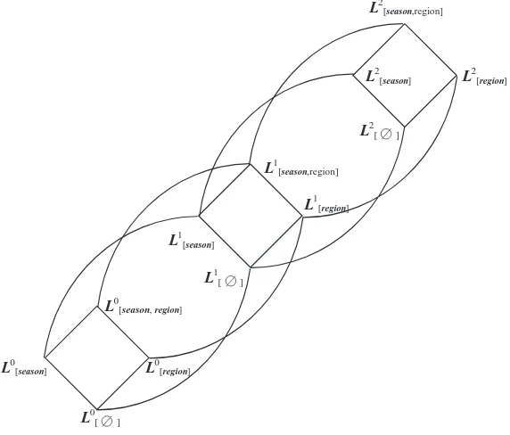
holds.). AllLk[A]succeeded byL2[season,region]are
orga-nized in the hierarchy shown inFig. 4.
Since d defines only a partial order over Lk[A],
there are many possible sequences in which they may be computed. Consider our running example of finding pairs of products bought frequently together in the same region and during the same season. One possibility is to first find all frequent products (L1[F]) Then, find frequent products for a particular
season (L1[season]), then frequent products for a
par-ticular season and region (L1[season,region]), and finally
pairs of products for a particular season and region
(L2[season,region]). Another possibility is to first find
frequent products for a particular region (L1[region]),
then frequent products for a particular season
(L1[season]), the frequent pairs of products (L
2 [F]), and
finally pairs of products for a particular season and region (L2[season,region]).
L2
[season,region]
L2
[season] L2[region]
L2[ ]
L1
[season,region]
L1[region]
L1 [season]
L1[ ]
L0
[season,region]
L0[season] L0[region]
L0[ ]
Note that there are no such alternatives when stan-dard association rules are used. Optimization techni-ques based on a-priori are essentially rule-based since the actual sizes of the initial data and intermediate result do not influence the sequence of steps. In fact, the sequence is always the same.
For qualified association rules, the sequence of steps is not always the same because of different possible alternatives as illustrated above. Intuitively, the source of alternatives is the fact that non-item dimensions are not symmetric and comparable.
Before we describe an algorithm for choosing an efficient sequence (in Section 6.2), we discuss the individual steps and their interaction within a sequence. The crux of our method (and of a-priori for that matter) is to use the result of a simpler query (which represents a portions of the entire query) to speed up the computation of the entire query. For example, if we are looking for pairs of item qualified by season and region (L2[season,region]), we can
elimi-nate all tuples from F that do not contribute to the computation of frequent items qualified by season
(L1[season]). Then, we can use the reduced fact table
to compute the qualified pairs. Generally, every step in our framework has two parts:
1. computeLk[A],
2. use the computed computeLk[A]to reduceF.
This framework is similar to query flocks[26]and can be adapted to handle iterative, candidate-growing, algorithms, such as a-priori [1]. Instead of reducing the size of the fact table in step 2, we can useLk[A]to
generate the new candidate set for the next iteration of the algorithm.
Next, we detail the two-part step and the interac-tion within a sequence.
3.3.1. Computing L[A]k
First, we expressLk[A]in relational algebra. Without
loss of generality, we assume that A= {A1,. . ., Am}
andAi is attribute of dimension tableDi.
rcount TIDð ÞN¼wðcIk;AðFkZEDJÞÞ
where Fk is a k-way self-join of the fact table F
on TID, Ik is a set of the keys (K0) of the item
dimension from each of the k copies of the fact
table, DJ is a cross product of D1,. . .,Dm, g is the aggregation operator, and w is the minimum support.
In SQL,Lk[A]can be computed as follows:
SELECT F1.K0,. . ., Fk.K0, A1,. . ., Am
FROM F AS F1,. . ., F AS Fk, D1,. . ., Dm WHERE F1.TID = F2.TID. . .
AND F1.TID = Fk.TID AND F1.K1 = D1.K1. . .
AND F1.Km = Dm.Km
GROUP BY F1.K0, . . ., Fk.K0, A1, . . ., Am
HAVING COUNT (DISTINCT F1.TID)N=:minsup
3.3.2. Reducing the fact table F with Lk[A]
First, consider the case whenk= 1 andA=FThen
L1[F], as a relation, has only one attribute,K0. The fact
table is reduced by semijoining it withL1[F]:
FZEprcount TIDð Þ
N¼w cK0ð ÞF
LetA= {A1,. . ., Am}. ThenL 1
[A]has, in addition to K0, attributesA1,. . ., Am. Therefore, the reduction of F has to involveDJ in addition toL1[A]:
FZEpðDJZErcount TIDð Þ
N¼wðcK0;AðFkZEDJÞÞÞ
In the general case, for kN1, where I1 is the
first attribute in Ik, we can express the reduction as
follows:
X ¼FkZEDJZErcount TIDð ÞN¼w cIk;AðFkZEDJÞ
F ZEpkTID;I
1;KI...;Kmð Þ:X
Intuitively, we need the TID in the last expression, in order to connect the items in the qualified itemsets.
3.3.3. Computing a sequence of Lk[A]
So far, we considered computingLk[A]individually.
In this section we consider, what happens when we compute several of them. In particular, we examine how to use a computedLk[A]to speed up the
computa-tion of another Ll[B]. We consider all three possible
cases:
!Lk[A]dLl[B]. In this case, using the computed set of
rea-son is thatLl[B]can be arbitrarily large regardless of
the sizeLk[A]. In an extreme caseLk[A]can be empty
and Ll[B]can be as large as possible.
!Lk[A]Ll[B]. This is the case that corresponds to the
condition in a-priori. The computed set can be used in computing Ll[B]as shown in a-priori.
!Lk[A] d Ll[B]. In this case, using an argument
similar to the first case, we can show that the computed set does not help.
Thus, the order of computation affects the actual result, so we will use a different notation to denote that the computation of the frequent qualified itemsets is happening in context of other computations. We defineRkAto be the computation ofLk[A]on thecurrent
reduced fact tableF:
RkA¼rcount TIDð ÞN¼w
cIk;A FkredZEDJ
whereFkred is ak-way self join of what remains of the
fact table after the previous reduction. For the first reductionFkred=Fk.
3.4. Optimization algorithm
We can show that the plan space for the optimi-zation problem is double-exponential in number of qualified dimensions. Consider all reducers at level 1. Since we have m dimensions and a reducer involves any subset of these dimensions, then the number of possible reducers is 2m. A plan involves any subset of all possible reducers, so the number of possible plans for one level is 22m. If we consider
n levels, then the total number of possible plans is 2n2m.
The number of possible reducers isn2mwheren is the maximum itemset size and m is the number of qualified dimensions. Since a plan is any subset of these reducers, the plan space is at least 2n2m.
The algorithm uses the following definitions. Let
RAk be a reducer and letP be a sequence of reducers.
Then we define the following:
!cost(RAk,P) as the cost of computing RkA after all
reducers in P have been computed and applied.
!frac(RAk,P) is the fraction of the fact table that is
reduced by applyingRkAafter all reducers inPhave
been applied.
We propose a greedy algorithm for finding a plan for computingRkA.
Input:RAk
Output:P begin
P=F
/*V contains all reducers succeeded by RkA
includingRkA */
V= {Rji|1 ViVk,Jp A} repeat
choose RBl fromV such that cost(RBl,P)/frac(RBl,P) is minimal.
append RBl toP
remove RBl fromV until(l=kandA=B)
returnP end
The algorithm starts with the full set of options to choose from: all reducers that are succeeded by RkA
and therefore can help in computingRkA. Then,
itera-tively, the reducer that has the smallest cost per unit of reduction is chosen until this reducer isRkA.
However, we can improve this algorithm in several ways. The first improvement is based on the following observation:
IfRkAePandRkAvRBl then,frac(RBl,P) = 0. Once a
reducer is applied, there is no further reduction by reducers dominated by the first one. Therefore, we can limit the set of possible choice V by removing all reducers dominated by the last chosen reducer.
The second improvement is to consider all reducers of each level separately. Such levelwise approach is appropriate for several reasons. First, it allows us to find all frequent qualified itemsets regardless of their size because we compute Li[A]for all i not justi=k.
Second, we can compute the confidence of a qualified association rule without an additional pass over the data. Third, it allows us to use better cost and reduc-tion estimates since we only compare reducer at the same level.
The greedy levelwise algorithm (improved as described) is shown below:
Input:RAk
P=F
fori= 1..k
V=RiJ |JpA} repeat
choose RlB from V such thatcost(RlB,P)/ frac(RlB,P) is minimal.
appendRlBtoP
removeRlB fromV
removeRlC fromV forC oB until(B=A)
returnP end
The algorithm tackles each level separately by applying the general greedy algorithm to the set of all reducers at each level.
3.5. Cost estimation
Finding closed formulas or even close estimates for cost (cost) and reduction (frac) functions is a hard problem. The information required in order to make the estimation tight can only be obtained after mining the data. Thus, we focus our attention on relatively simple models that lead to the selection of efficient plans by the levelwise greedy algorithm. In our future work, we will consider using the mining results from previous queries to make even better estimates.
First, let us consider the cost function:cost(RkA,P)
and letA= {A1,. . ., Am}, where Ai is attribute of Di.
Let the size of the fact table befand the sizes of the dimension tables bedi. Recall that there are two steps
of each reduction: computing and applying the redu-cer. The reducer is computed as follows:
rcount TIDð ÞN¼w
cIk;AðFkZEDJÞÞ:
Before we tackle the general case, consider the case when k= 1 andA=F. Then we can rewrite the expression as follows:
rcount TIDð ÞN¼w cK0ð ÞF
:
The cost of this expression is the cost of accessing and aggregating F. Since most database systems implement aggregation using sorting, and sorting requires reading F a small number of times (e.g. using two phase merge sort) the cost is linear in f. Consider the case when k= 1 and A is not empty.
Then the expression can be written as:
rcount TIDð ÞN¼w
cK0;A1;...;AmðFZED1ZE. . .ZEDmÞÞ:
Because of the star schema every tuple inF joins with exactly one tuple from each Di. Thus, we can
estimate the cost of this reducer is linear in thesumof the sizes of the dimension tables. In the general case it is difficult to estimate the size of Fk. Fortunately in
the levelwise greedy algorithm we only compare reducers at the same level so the exact value is not important.
Since the cost is linear in the size of the fact table and in thesumof the sizes of the dimension tables, the formula for the cost is:
cost R kA;P¼c1fk
Xm
i¼1
2diþsizeof RkA;P
!
þc2
where c1andc2are system dependent constants. We
count eachditwice because both the computation and
application ofRkAinvolve dimension tableDiwhereas RkA is used only in the application.
Next we estimate the fraction function that also determinessizeof(RkA,P) we need to estimate the
num-ber of different qualified itemsets that are frequent. The estimate of the fraction of all tuples in the fact table that will be eliminated by a reducer RkA
depends crucially on the distribution of the values in
F. The simple assumption that this distribution is uniform leads to straightforward calculations and has been used successfully in optimizing join ordering and view materialization. In our case, however, the uniformity assumption is clearly at odds with the goal of mining associations. In fact, mining associa-tion-rules is meaningless for uniformly distributed data since any combination is equally likely. Recent research has shown empirically [5] that large data-sets, especially transaction-based ones, tend to have a skewed distribution that can be approximated by the Zipfian distribution. The Zipfian distribution is characterized by the property that the number of occurrences of each value is inversely proportional to its rank. Thus, if the most frequent value occurs x
times, then the n-th most frequent value occurs x/n
First, consider the simplest case whenk= 1 and A
is empty. Let the number of different items (values of attributek0) that occur inFbep=domain(K0), and let
the size of F be f. Then, if the most frequent item occurs x times, we have the approximate equality:
xX
p
i¼1 1
icf:
The sum of the first p members of the harmonic series can be approximated by lnp+ 0.577. Then, we have:
xc f
lnpþ0:577:
If the minimum support threshold is w, then the number of items that occur at leastwtimes is approxi-mately y(the y most frequent ones), wherex/ycw. Substituting forxwe get the formula fory:
yc f
wðlnpþ0:577Þ:
Note thatsizeof(R1F, P)) =y. The y most frequent
items appear in approximately xPy
i¼11i tuples of f.
Thus, we can derivefrac(R1F,F) as follows:
1
xX
y
i¼1 1
i
f :
After substituting the values of xand y and alge-braic manipulation we get:
frac R1F;F
c
lnpwðlnpþ0:577Þ
f
lnpþ0:577 :
Let us consider the case when k= 1 and A= {A1,. . ., Am}. We shall assume that values of the tuple K0, A1,. . ., Amfollow a Zipfian distribution. Thus, we can
apply the above formula with a differentp: the num-ber of different combinations of values ofK0,A1,. . ., Am that occur in the data. Without any additional
information we can assume that all combinations are possible but their number cannot exceed the number of tuples inF. Thus, in this casep=min(domain(K0)
jmi¼1 domain(Ai),f).
In general, forkN1, the computation of the fraction function is much more complex. We will show how to
reduce the casek= 2 to an approximately equivalent case with k= 1. Using a composition of k1 such reductions we can reduce the case for anykN1 to the case k= 1. Recall that the last reducer computed and applied by the levelwise greedy algorithm (described in Section 6.2) at level 1 is R1A. By running several
simple queries over R1A we can find the number of
different values in the reduced fact table F for any attribute Ai, i.e. the new domain(Ai). Also, we can
find the number of different items (values ofK0), the
total number of tuples left and the total number of transactions. Thus, we can estimate the average num-ber of items per transactions and the total numnum-ber of pairs of items, which is the size of F2, where F2=F./TID = TID F. Consider the non-materialized
table F2 and consider a pair of items to be a new
item. Each reducer at level 2 acts as a level 1 reducer for this new table and items. We assume that a reduc-tion of the new table of pairs will correspond to the same reduction of F. Therefore, we can use the method outlined fork= 1 in this situations. Note that we use this method only to choose the reducers at level 2; not to implement them. These reducers are applied to the fact table F; not the table of pairs. So far, we derived formulas only forfrac(RkA,F).
Now we consider the interaction among different redu-cers. Suppose RkA is chosen first. We need to define frac(RBk, {RkA}). We consider the three possible cases:
!AsB.ThenLk[A]dLk[B]and therefore the fraction
is 0. For example, eliminating all tuples with non-frequent items, after eliminating all tuples with non-frequent items qualified with a season, does not help at all.
!AoB.ThenLk[A]Lk[B]and thus any tuple
elimi-nated by the second reducer is also elimielimi-nated by the first. Therefore: frac(RkB, {RkA}) = (frac(RkB,
F)frac(RkA,F)) / (1frac(RkA,F).
!AKBKA. In this case, the exact value cannot be determined but we can get an estimate as follows. Let the fraction of tuples eliminated by both RkA
and RkB be z; and let frac(RkA, F) = fA, frac(RkB,
F) = fB, and frac(RAk[B,F) = fAB. The following
contingency table reflects the constraints we have:
reduced byRk
B not byRkB
byRk
A z fAz
not byRk
Without any additional information a good esti-mate forz is in the middle of the range of possible values given by:
Thus, we determine how to update thefrac func-tion after any reducer is computed and applied which is needed by the optimization algorithm.
4. Experiments and performance
For our experiments we used Oracle 9i RDBMS running under SunOS 5.9. We used subsets of data from a 23 terabytes corporate data warehouse that
stores data for a major US-based retailer over 2-year period. In our experiments we mined both association rules and qualified association rules. In this paper, we present the results of queries that are typical for our experiments.
Our first experiment consists of two queries and it uses a schema that is nearly equivalent to the schema shown inFig. 1, with one difference being the absence of the customer dimension. The first query finds regular association rules based on the following question:
Find all pairs of items that appear together in more
than 1500 transactions.
The implementation of this query involves pruning of all items that do not appear in more than 1500 transactions. The result of the query is more than 1500 pairs of items. We show the 20 most frequent ones in
Table 3.
The second query finds qualified association rules and is based on the following question
Find all pairs of items that appear together in more than 1500 transactions in the same region during the same month.
The implementation of this query involves pruning all item-region pairs that do not appear in more than 1500 transactions. The result of this query, shown in
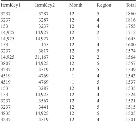
Table 4, is a set of eighteen rules, where each rule involves two items, a month, and a region. The rules are ordered by frequency (the most frequent appears at the top of the table).
Table 3
US retailer-associations rules found (top 20 with highest support)
ItemKey1 ItemKey2 Total
US retailer—qualified associations rules found
ItemKey1 ItemKey2 Month Region Total
3237 3287 12 5 1860
3237 3287 12 4 1816
153 3237 12 4 1755
14,925 14,927 12 2 1712
14,925 14,927 12 1 1645
153 155 12 4 1600
3237 3817 12 5 1574
14,925 31,167 12 2 1564
3807 14,925 12 5 1557
3237 4519 12 5 1549
4519 4769 1 4 1543
4519 4769 1 5 1537
153 3287 12 4 1535
153 14,925 12 4 1524
3237 3567 12 4 1521
3237 3441 12 5 1515
4835 14,925 12 5 1505
When we compare the two tables, we first notice that by and large they contain different itemsets. For example, compare the top two pairs in each set (31,107, 31,167—Table 3 and 3237, 3287—Table 4). The pair (3237, 3287) is not in the top 20 frequent pairs; however, when month and region are qualified it stands out as the most frequent pair (for Region 5
andDecember). On the other hand, the pair (31,107,
31,167) is the most frequent pair overall but when month and region are qualified this pair is not fre-quent, for any month and region combination.
This experiment illustrates that qualified associa-tion rules can reveal addiassocia-tional valuable informaassocia-tion that would not have been discovered using standard association rules mining. In this case standard asso-ciation rules find the correlated sales that are spread among many markets and months (which may be used, for example, when planning a long-term nationwide or global marketing campaign), while qualified association rules find the correlated sales
that are concentrated in particular markets over par-ticular time periods (which may be used, for exam-ple, when planning a series of shorter term marketing campaigns with regional focus). As shown in this real-world example, the standard and qualified rules can involve completely different sets of items.
In our second experiment, we compared the num-ber of discovered qualified association rules with the number of standard association rules mined from the same set, while varying the value of minimum sup-port. The results are shown inTable 5.
As expected, for lower values of minimum sup-port, the number of standard rules is overwhelming (examining and making decisions based on thou-sands of rules is usually not realistic), while the number of qualified rules is still manageable. Furthermore, for lower values of minimum support, the cost of finding all standard rules is extremely high, because the first step of a-priori results in a very small reduction of the possible pairs of items. This observation supports our argument (stated in 4.1) that it is not feasible to use standard association rule mining to find qualified rules, by simply con-sidering value of each qualifier as just another item added to the transaction.
Table 5
The number of discovered standard and qualified association rules
Minimum support (000) 20 10 5 2 1.5 1 .5 No. of qualified rules 0 0 0 0 18 255 3231 No. of standard rules 8 105 more than 5000
100 1000 10000 100000
200 400 600 800 1000 1200 1400 1600 1800 2000 2200 2400 2600 2800 3000 3200 3400 3600 3800
Minimum Support (number of transactions)
Cost (Estimate)
0 Region Season Season, Region
4000 4200 4400 4600 4800
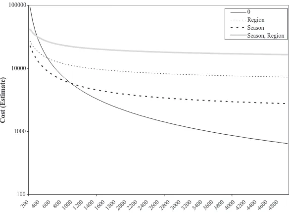
Our next set of experiments focuses on the optimi-zation process and performance. We detail our fin-dings for the mining problem of finding frequent pairs of items qualified by season and regionL2[season,region].
First, we considered how the first step of the plan picked by the greedy algorithm changes with respect to the minimum support, as shown inFig. 5.
When the support was relatively low, less than 1000, the first step that was chosen was R1season
month. For support greater than 1000, R1F is the
winner. These results confirm our intuition, since for higher support the expected reduction from conside-ring just items is significant, whereas for low mini-mum support this reduction is negligible and offsets the lower cost ofR1F.
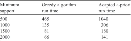
Finally, we compared the performance of the plan picked by the levelwise greedy algorithm against the fixed plan that corresponds to the second mapping of qualified association rules to standard association rules as described in Section 3.2 (we chose the second mapping as a representative; similar conclusions would hold for the comparison with both the same conclusions would hold for first and third mapping). As we mentioned in Section 3.2, approaches based on standard association rule mining, could be used, in theory, to find qualified association rules. However, the performance cost for such approaches is signifi-cantly higher than the cost of our approach, which is designed especially for finding qualified association rules. This is illustrated by the performance numbers summarized inTable 6.
While the actual numbers are system dependent, our algorithm clearly outperforms the statically cho-sen sequence corresponding to bundling together item, region and dimension. The main reason for the stark difference in performance is that the bundling precludes any opportunities for reduction which is
crucial in speeding up the first few steps of the sequence of reducers.
5. Conclusions
In this paper, we presented a new data-mining framework, called qualified association rules, that is tightly integrated with database technology. We showed how qualified association rules can enable organizations to find new information within their data warehouses relatively easily, utilizing their exis-ting technology.
We were motivated by the observation that exis-ting association-rule based approaches are capable of effectively mining data warehouse fact tables in con-junction with the item-related dimension only. We introduced qualified association rules as a method for mining fact tables as they relate to the attributes from both item and non-item dimensions. Standard association rules find coarser granularity correlations among items while qualified rules discover finer patterns. Both types of rules can provide valuable insight for the organization that owns the data. Com-bined information, extrapolated by examining both
standard and qualified association rules, is much
more likely to truly reveal the nature of the data stored in the corporate data warehouse and the knowledge captured in it. The existing methods are suited to provide only partial information (standard rules) from data warehouses and, in most cases, require that the data must be retrieved from the database repository and examined by using separate software. Our method provides a more complete view of the data (both standard and qualified rules), while allowing the data to remain in the data ware-house and using the processing power of the database engine itself. State-of-the-art RDBMS query optimi-zers cannot handle mining qualified association rules directly. Our approach, using an external optimizer, leverages their strength and works around their weak-nesses, thus making the mining processing effective and efficient.
Besides integrated analytical data collections, such as data warehouses or data marts, many other data repositories are organized in a dimensional-like fash-ion. For example, it is very common for regular operational databases and files to include tables that Table 6
Running times for the plans produced by the greedy algorithm and the static a-priori plan
Minimum support
Greedy algorithm run time
Adapted a-priori run time
500 465 1040
1000 135 306
1500 81 180