with MA
TLAB® Applications
Signals and
Systems
Steven T. Karris
Orchard Publications www.orchardpublications.com
Second Edition
Includes
step-by-step
procedures
for designing
analog and
digital filters
X m[ ] x n[ ]e
j2πm n N ---–
n=0 N 1–
Orchard Publications, Fremont, California Visit us on the Internet
www.orchardpublications.com or email us: [email protected]
Signals and Systems
with MATLAB® Applications
Second Edition
Steven T. Karris
Second Edition, to be a concise and easy-to-learn text. It provides complete, clear, and detailed expla-nations of the principal analog and digital signal processing concepts and analog and digital filter design illustrated with numerous practical examples.
This text includes the following chapters and appendices:
• Elementary Signals • The Laplace Transformation • The Inverse Laplace Transformation • Circuit Analysis with Laplace Transforms • State Variables and State Equations • The Impulse Response and Convolution • Fourier Series • The Fourier Transform • Discrete Time Systems and the Z Transform • The DFT and The FFT Algorithm • Analog and Digital Filters
• Introduction to MATLAB • Review of Complex Numbers • Review of Matrices and Determinants
Each chapter contains numerous practical applications supplemented with detailed instructions for using MATLAB to obtain quick solutions.
Steven T. Karris is the president and founder of Orchard Publications. He earned a bachelors degree in electrical engineering at Christian Brothers University, Memphis, Tennessee, a mas-ters degree in electrical engineering at Florida Institute of Technology, Melbourne, Florida, and has done post-master work at the latter. He is a registered professional engineer in California and Florida. He has over 30 years of professional engineering experience in industry. In addi-tion, he has over 25 years of teaching experience that he acquired at several educational insti-tutions as an adjunct professor. He is currently with UC Berkeley Extension.
ISBN 0-9709511-8-3
Signals and Systems
with MATLAB® Applications
Second Edition
Steven T. Karris
Copyright © 2003 Orchard Publications. All rights reserved. Printed in the United States of America. No part of this publication may be reproduced or distributed in any form or by any means, or stored in a data base or retrieval system, without the prior written permission of the publisher.
Direct all inquiries to Orchard Publications, 39510 Paseo Padre Parkway, Fremont, California 94538
Product and corporate names are trademarks or registered trademarks of the Microsoft™ Corporation and The MathWorks™ Inc. They are used only for identification and explanation, without intent to infringe.
Library of Congress Cataloging-in-Publication Data
Library of Congress Control Number: 2003091595
ISBN 0-9709511-8-3
Preface
This text contains a comprehensive discussion on continuous and discrete time signals and systems with many MATLAB® examples. It is written for junior and senior electrical engineering students, and for self-study by working professionals. The prerequisites are a basic course in differential and integral calculus, and basic electric circuit theory.
This book can be used in a two-quarter, or one semester course. This author has taught the subject material for many years at San Jose State University, San Jose, California, and was able to cover all material in 16 weeks, with 2½ lecture hours per week.
To get the most out of this text, it is highly recommended that Appendix A is thoroughly reviewed. This appendix serves as an introduction to MATLAB, and is intended for those who are not familiar with it. The Student Edition of MATLAB is an inexpensive, and yet a very powerful software package; it can be found in many college bookstores, or can be obtained directly from
The MathWorks™ Inc., 3 Apple Hill Drive , Natick, MA 01760-2098 Phone: 508 647-7000, Fax: 508 647-7001
http://www.mathworks.com e-mail: [email protected]
The elementary signals are reviewed in Chapter 1 and several examples are presented. The intent of this chapter is to enable the reader to express any waveform in terms of the unit step function, and subsequently the derivation of the Laplace transform of it. Chapters 2 through 4 are devoted to Laplace transformation and circuit analysis using this transform. Chapter 5 discusses the state variable method, and Chapter 6 the impulse response. Chapters 7 and 8 are devoted to Fourier series and transform respectively. Chapter 9 introduces discrete-time signals and the Z transform.
Considerable time was spent on Chapter 10 to present the Discrete Fourier transform and FFT with the simplest possible explanations. Chapter 11 contains a thorough discussion to analog and digital filters analysis and design procedures. As mentioned above, Appendix A is an introduction to MATLAB. Appendix B contains a review of complex numbers, and Appendix C discusses matrices.
New to the Second Edition
This is an refined revision of the first edition. The most notable changes are chapter-end summaries, and detailed solutions to all exercises. The latter is in response to many students and working professionals who expressed a desire to obtain the author’s solutions for comparison with their own. The author has prepared more exercises and they are available with their solutions to those instructors who adopt this text for their class.
Orchard Publications Fremont, California
Table of Contents
Chapter 1
Elementary Signals
Signals Described in Math Form ...1-1 The Unit Step Function ...1-2 The Unit Ramp Function ...1-10 The Delta Function ...1-12 Sampling Property of the Delta Function...1-12 Sifting Property of the Delta Function...1-13 Higher Order Delta Functions...1-15 Summary...1-19 Exercises...1-20 Solutions to Exercises ...1-21
Chapter 2
The Laplace Transformation
Definition of the Laplace Transformation... 2-1 Properties of the Laplace Transform... 2-2 The Laplace Transform of Common Functions of Time ...2-12 The Laplace Transform of Common Waveforms ...2-23 Summary...2-29 Exercises...2-34 Solutions to Exercises ...2-37
Chapter 3
The Inverse Laplace Transformation
The Inverse Laplace Transform Integral...3-1 Partial Fraction Expansion ...3-1 Case where is Improper Rational Function ( )... 3-13 Alternate Method of Partial Fraction Expansion... 3-15 Summary... 3-18
Exercises ...3-20 Solutions to Exercises ...3-22
Chapter 4
Circuit Analysis with Laplace Transforms
Circuit Transformation from Time to Complex Frequency...4-1 Complex Impedance ...4-8 Complex Admittance ...4-10 Transfer Functions ...4-13 Summary ...4-16 Exercises ...4-18 Solutions to Exercises ...4-21
Chapter 5
State Variables and State Equations
Expressing Differential Equations in State Equation Form... 5-1 Solution of Single State Equations... 5-7 The State Transition Matrix ... 5-9 Computation of the State Transition Matrix ...5-11 Eigenvectors ...5-18 Circuit Analysis with State Variables ...5-22 Relationship between State Equations and Laplace Transform...5-28 Summary ...5-35 Exercises ...5-39 Solutions to Exercises ...5-41
Chapter 6
The Impulse Response and Convolution
The Impulse Response in Time Domain... 6-1 Even and Odd Functions of Time...6-5 Convolution... 6-7 Graphical Evaluation of the Convolution Integral ...6-8 Circuit Analysis with the Convolution Integral... 6-18 Summary ... 6-20
Z s( )
Exercises... 6-22 Solutions to Exercises ... 6-24
Chapter 7
Fourier Series
Wave Analysis...7-1 Evaluation of the Coefficients ...7-2 Symmetry...7-7 Waveforms in Trigonometric Form of Fourier Series ... 7-11 Gibbs Phenomenon... 7-24 Alternate Forms of the Trigonometric Fourier Series ... 7-25 Circuit Analysis with Trigonometric Fourier Series ... 7-29 The Exponential Form of the Fourier Series ... 7-31 Line Spectra ... 7-35 Computation of RMS Values from Fourier Series ... 7-40 Computation of Average Power from Fourier Series ... 7-42 Numerical Evaluation of Fourier Coefficients... 7-44 Summary... 7-48 Exercises... 7-51 Solutions to Exercises ... 7-53
Chapter 8
The Fourier Transform
Chapter 9
Discrete Time Systems and the
Z
Transform
Definition and Special Forms ... 9-1 Properties and Theorems of the
Z
Tranform ... 9-3 TheZ
Transform of Common Discrete Time Functions...9-11Computation of the
Z
transform with Contour Integration ...9-20Transformation Between and Domains...9-22 The Inverse
Z
Transform...9-24The Transfer Function of Discrete Time Systems ...9-38 State Equations for Discrete Time Systems ...9-43 Summary ...9-47 Exercises ...9-52 Solutions to Exercises ...9-54
Chapter 10
The DFT and the FFT Algorithm
The Discrete Fourier Transform (DFT) ...10-1 Even and Odd Properties of the DFT...10-8 Properties and Theorems of the DFT... 10-10 The Sampling Theorem ... 10-13 Number of Operations Required to Compute the DFT... 10-16 The Fast Fourier Transform (FFT) ... 10-17 Summary ... 10-28 Exercises ... 10-31 Solutions to Exercises ... 10-33
Chapter 11
Analog and Digital Filters
Filter Types and Classifications ... 11-1 Basic Analog Filters... 11-2 Low-Pass Analog Filters... 11-7 Design of Butterworth Analog Low-Pass Filters ... 11-11 Design of Type I Chebyshev Analog Low-Pass Filters... 11-22 Other Low-Pass Filter Approximations... 11-34 High-Pass, Band-Pass, and Band-Elimination Filters... 11-39
Digital Filters ... 11-49 Summary... 11-69 Exercises... 11-73 Solutions to Exercises ... 11-79
Appendix A
Introduction to MATLAB®
MATLAB® and Simulink®...A-1
Command Window...A-1 Roots of Polynomials ...A-3 Polynomial Construction from Known Roots...A-4 Evaluation of a Polynomial at Specified Values...A-6 Rational Polynomials ...A-8 Using MATLAB to Make Plots ...A-10 Subplots ...A-18 Multiplication, Division and Exponentiation ...A-18 Script and Function Files...A-25 Display Formats ...A-30
Appendix B
Review of Complex Numbers
Definition of a Complex Number... B-1 Addition and Subtraction of Complex Numbers... B-2 Multiplication of Complex Numbers... B-3 Division of Complex Numbers ... B-4 Exponential and Polar Forms of Complex Numbers ... B-4
Appendix C
Matrices and Determinants
Chapter 1
Elementary Signals
his chapter begins with a discussion of elementary signals that may be applied to electric net-works. The unit step, unit ramp, and delta functions are introduced. The sampling and sifting properties of the delta function are defined and derived. Several examples for expressing a vari-ety of waveforms in terms of these elementary signals are provided.
1.1 Signals Described in Math Form
Consider the network of Figure 1.1 where the switch is closed at time .
Figure 1.1. A switched network with open terminals.
We wish to describe in a math form for the time interval . To do this, it is conve-nient to divide the time interval into two parts, , and .
For the time interval , the switch is open and therefore, the output voltage is zero. In other words,
(1.1)
For the time interval , the switch is closed. Then, the input voltage appears at the output, i.e.,
(1.2)
Combining (1.1) and (1.2) into a single relationship, we get
(1.3)
We can express (1.3) by the waveform shown in Figure 1.2.
T
t = 0
+− +
−
vout
vS t = 0
R
open terminals
vout –∞< <t +∞
∞< <t 0
– 0< <t ∞
∞< <t 0
– vout
vout = 0 for –∞< <t 0
0< <t ∞ vS
vout = vS for 0< <t ∞
vout 0 –∞< <t 0 vS 0< <t ∞
⎩ ⎨ ⎧ =
Figure 1.2. Waveform for as defined in relation (1.3)
The waveform of Figure 1.2 is an example of a discontinuous function. A function is said to be
dis-continuous if it exhibits points of discontinuity, that is, the function jumps from one value to another
without taking on any intermediate values.
1.2 The Unit Step Function
A well-known discontinuous function is the unit step function * that is defined as
(1.4)
It is also represented by the waveform of Figure 1.3.
Figure 1.3. Waveform for
In the waveform of Figure 1.3, the unit step function changes abruptly from to at . But if it changes at instead, it is denoted as . Its waveform and definition are as shown in Figure 1.4 and relation (1.5).
Figure 1.4. Waveform for
* In some books, the unit step function is denoted as , that is, without the subscript 0. In this text, however, we will reserve the designation for any input when we discuss state variables in a later chapter.
0
vout
vS
t
vout
u
0( )
t
u0( )t
u t( ) u t( )
u0( )t 0 t<0
1 t>0
⎩ ⎨ ⎧ =
u0( )t
0 1
t
u0( )t
u0( )t 0 1 t = 0
t = t0 u0(t–t0)
1
t0 0
u0(t–t0)
t
The Unit Step Function
(1.5)
If the unit step function changes abruptly from to at , it is denoted as . Its
waveform and definition are as shown in Figure 1.5 and relation (1.6).
Figure 1.5. Waveform for
(1.6)
Example 1.1
Consider the network of Figure 1.6, where the switch is closed at time .
Figure 1.6. Network for Example 1.1
Express the output voltage as a function of the unit step function, and sketch the appropriate waveform.
Solution:
For this example, the output voltage for , and for . Therefore,
(1.7)
and the waveform is shown in Figure 1.7.
u0(t–t0) 0 t<t0
1 t>t0
⎩ ⎨ ⎧ =
0 1 t = –t0 u0(t+t0)
t −t0 0
1 u0(t+t0)
u0(t+t0)
u0(t+t0) 0 t t0
– <
1 t>–t0
⎩ ⎨ ⎧ =
t = T
+− +
−
vout
vS t = T
R
open terminals
vout
vout = 0 t<T vout = vS t>T
Figure 1.7. Waveform for Example 1.1
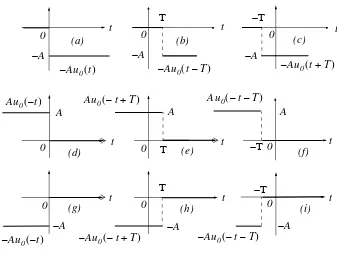
Other forms of the unit step function are shown in Figure 1.8.
Figure 1.8. Other forms of the unit step function
Unit step functions can be used to represent other time-varying functions such as the rectangular pulse shown in Figure 1.9.
Figure 1.9. A rectangular pulse expressed as the sum of two unit step functions
Thus, the pulse of Figure 1.9(a) is the sum of the unit step functions of Figures 1.9(b) and 1.9(c) is
represented as .
T t
0
vSu0(t–T)
vout
0 t
t
t t
Τ −Τ
0
0 0
0 Τ
0
0
t
t t
0 t 0 t
−Τ
−Τ Τ
(a) (b) (c)
(d) (e) (f)
(g) (h) (i)
−A −A −A
−A −A −A
A A A
Au0( )–t
A
– u0( )t –Au0(t–T) –Au0(t+T)
Au0(–t+T) Au0(–t–T)
A
– u0( )–t –Au0(–t+T) –Au0(–t–T)
0 1 t 0 t 0 t
1
1 u0 t
( )
u0(t–1)
–
a
( ) ( )b ( )c
The Unit Step Function
The unit step function offers a convenient method of describing the sudden application of a voltage or current source. For example, a constant voltage source of applied at , can be denoted
as . Likewise, a sinusoidal voltage source that is applied to a circuit at
, can be described as . Also, if the excitation in a circuit is a
rect-angular, or trirect-angular, or sawtooth, or any other recurring pulse, it can be represented as a sum (dif-ference) of unit step functions.
Example 1.2
Express the square waveform of Figure 1.10 as a sum of unit step functions. The vertical dotted lines indicate the discontinuities at and so on.
Figure 1.10. Square waveform for Example 1.2
Solution:
Line segment { has height , starts at , and terminates at . Then, as in Example 1.1, this segment is expressed as
(1.8)
Line segment | has height ,starts at and terminates at . This segment is expressed as
(1.9)
Line segment } has height , starts at and terminates at . This segment is expressed as
(1.10)
Line segment ~ has height ,starts at , and terminates at . It is expressed as
(1.11)
Thus, the square waveform of Figure 1.10 can be expressed as the summation of (1.8) through (1.11), that is,
24V t = 0
24u0( )t V v t( ) = Vmcosωt V
t = t0 v t( ) = (Vmcosωt)u0(t–t0) V
T 2T 3T, ,
{
|
}
~
t v t( )
3T A
0
A
–
T 2T
A t = 0 t = T
v1( )t = A u[ 0( )t –u0(t–T)]
A
– t = T t = 2T
v2( )t = –A[u0(t–T)–u0(t–2T)]
A t = 2T t = 3T
v3( )t = A u[ 0(t–2T)–u0(t–3T)]
A
– t = 3T t = 4T
(1.12)
Combining like terms, we get
(1.13)
Example 1.3
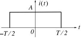
Express the symmetric rectangular pulse of Figure 1.11 as a sum of unit step functions.
Figure 1.11. Symmetric rectangular pulse for Example 1.3
Solution:
This pulse has height , starts at , and terminates at . Therefore, with reference to Figures 1.5 and 1.8 (b), we get
(1.14)
Example 1.4
Express the symmetric triangular waveform of Figure 1.12 as a sum of unit step functions.
Figure 1.12. Symmetric triangular waveform for Example 1.4
Solution:
We first derive the equations for the linear segments { and | shown in Figure 1.13.
The Unit Step Function
Figure 1.13. Equations for the linear segments of Figure 1.12
For line segment {,
(1.15)
and for line segment |,
(1.16)
Combining (1.15) and (1.16), we get
(1.17)
Example 1.5
Express the waveform of Figure 1.14 as a sum of unit step functions.
Figure 1.14. Waveform for Example 1.5.
Solution:
Figure 1.15. Equations for the linear segments of Figure 1.14
Following the same procedure as in the previous examples, we get
Multiplying the values in parentheses by the values in the brackets, we get
or
and combining terms inside the brackets, we get
(1.18)
Two other functions of interest are the unit ramp function, and the unit impulse or delta function. We will introduce them with the examples that follow.
Example 1.6
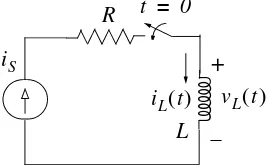
In the network of Figure 1.16 is a constant current source and the switch is closed at time .
Figure 1.16. Network for Example 1.6
1 2 3
1 2 3
0 {
|
2t+1
v t( )
t t
– +3
v t( ) = (2t+1)[u0( )t –u0(t–1)]+3 u[ 0(t–1)–u0(t–2)]
+ (–t+3)[u0(t–2)–u0(t–3)]
v t( ) = (2t+1)u0( )t –(2t+1)u0(t–1)+3u0(t–1)
3u0(t–2)
– +(–t+3)u0(t–2)–(–t+3)u0(t–3)
v t( ) = (2t+1)u0( )t +[–(2t+1)+3]u0(t–1)
+ [–3+(–t+3)]u0(t–2)–(–t+3)u0(t–3)
v t( ) = (2t+1)u0( )t –2 t( –1)u0(t–1)–tu0(t–2)+(t–3)u0(t–3)
iS t = 0
vC( )t
t = 0
iS
R
C −
The Unit Step Function
Express the capacitor voltage as a function of the unit step.
Solution:
The current through the capacitor is , and the capacitor voltage is
* (1.19)
where is a dummy variable.
Since the switch closes at , we can express the current as
(1.20)
and assuming that for , we can write (1.19) as
(1.21)
or
(1.22)
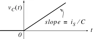
Therefore, we see that when a capacitor is charged with a constant current, the voltage across it is a linear function and forms a ramp with slope as shown in Figure 1.17.
Figure 1.17. Voltage across a capacitor when charged with a constant current source.
* Since the initial condition for the capacitor voltage was not specified, we express this integral with at the lower limit of integration so that any non-zero value prior to would be included in the integration.
1.3 The Unit Ramp Function
The unit ramp function, denoted as , is defined as
(1.23)
where is a dummy variable.
We can evaluate the integral of (1.23) by considering the area under the unit step function from as shown in Figure 1.18.
Figure 1.18. Area under the unit step function from
Therefore, we define as
(1.24)
Since is the integral of , then must be the derivative of , i.e.,
(1.25)
Higher order functions of can be generated by repeated integration of the unit step function. For example, integrating twice and multiplying by 2, we define as
(1.26)
Similarly,
(1.27)
and in general,
The Unit Ramp Function
Figure 1.19. Network for Example 1.7
Express the inductor current in terms of the unit step function.
Solution:
The voltage across the inductor is
(1.30)
and since the switch closes at ,
(1.31)
Therefore, we can write (1.30) as
(1.32)
But, as we know, is constant ( or ) for all time except at where it is discontinuous. Since the derivative of any constant is zero, the derivative of the unit step has a non-zero value only at . The derivative of the unit step function is defined in the next section.
1.4 The Delta Function
The unit impulse or delta function, denoted as , is the derivative of the unit step . It is also
defined as
(1.33)
and
(1.34)
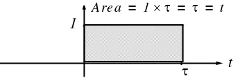
To better understand the delta function , let us represent the unit step as shown in Figure 1.20 (a).
Figure 1.20. Representation of the unit step as a limit.
The function of Figure 1.20 (a) becomes the unit step as . Figure 1.20 (b) is the derivative of Figure 1.20 (a), where we see that as , becomes unbounded, but the area of the rectangle remains . Therefore, in the limit, we can think of as approaching a very large spike or impulse at the origin, with unbounded amplitude, zero width, and area equal to .
Two useful properties of the delta function are the sampling property and the sifting property.
1.5 Sampling Property of the Delta Function
The sampling property of the delta function states that
(1.35)
or, when ,
(1.36)
δ
( )
t
δ( )t u0( )t
δ τ( ) τd ∞ –
t
∫
= u0( )tδ( )t = 0 for all t≠0
δ( )t u0( )t
−ε ε
1
2ε
Figure (a)
Figure (b) Area =1
ε
−ε
1
t
t 0
0
ε→0
ε→0 1 2⁄ ε
1 δ( )t
1
δ
( )
t
f t( )δ(t–a) = f a( )δ( )t
a = 0
Sifting Property of the Delta Function
that is, multiplication of any function by the delta function results in sampling the function at the time instants where the delta function is not zero. The study of discrete-time systems is based on this property.
Proof:
Since then,
(1.37)
We rewrite as
(1.38)
Integrating (1.37) over the interval and using (1.38), we get
(1.39)
The first integral on the right side of (1.39) contains the constant term ; this can be written out-side the integral, that is,
(1.40)
The second integral of the right side of (1.39) is always zero because
and
Therefore, (1.39) reduces to
(1.41)
Differentiating both sides of (1.41), and replacing with , we get
(1.42)
1.6 Sifting Property of the Delta Function
The sifting property of the delta function states that
(1.43)
that is, if we multiply any function by , and integrate from , we will obtain the value of evaluated at .
Proof:
Let us consider the integral
(1.44)
We will use integration by parts to evaluate this integral. We recall from the derivative of products that
(1.45)
and integrating both sides we get
(1.46)
Now, we let ; then, . We also let ; then, . By
substitu-tion into (1.46), we get
(1.47)
We have assumed that ; therefore, for , and thus the first term of the
right side of (1.47) reduces to . Also, the integral on the right side is zero for , and there-fore, we can replace the lower limit of integration by . We can now rewrite (1.47) as
Higher Order Delta Functions
1.7 Higher Order Delta Functions
An nth-orderdelta function is defined as the derivative of , that is,
(1.49)
The function is called doublet, is called triplet, and so on. By a procedure similar to the derivation of the sampling property of the delta function, we can show that
(1.50)
Also, the derivation of the sifting property of the delta function can be extended to show that
(1.51)
Example 1.8
Evaluate the following expressions:
a.
b.
c.
Solution:
a. The sampling property states that For this example, and
. Then,
b. The sifting property states that . For this example, and .
Then,
c. The given expression contains the doublet; therefore, we use the relation
Then, for this example,
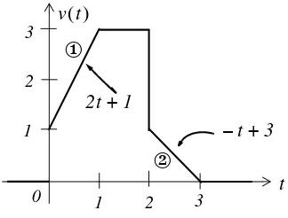
Example 1.9
a. Express the voltage waveform shown in Figure 1.21 as a sum of unit step functions for the
time interval .
b. Using the result of part (a), compute the derivative of and sketch its waveform.
Figure 1.21. Waveform for Example 1.9
Solution:
a. We first derive the equations for the linear segments of the given waveform. These are shown in Figure 1.22.
Next, we express in terms of the unit step function , and we get
(1.52)
Multiplying and collecting like terms in (1.52), we get
f t( )δ'(t–a) = f a( )δ'(t–a)–f'( )δa (t–a)
t2δ'(t–3) t2t=3δ'(t–3) d
dt
---t2 t=3δ(t–3)
– =
9δ'(t–3)–6δ(t–3)
=
v t( ) 1< <t 7 s
–
v t( )
−1
−2
−1 1 2 3
1 2 3 4 5 6 7
0
V
( )
t ( )s
v t( )
v t( ) u0( )t
v t( ) = 2t u[ 0(t+1)–u0(t–1)]+2 u[ 0(t–1)–u0(t–2)]
+ (–t+5)[u0(t–2)–u0(t–4)]+[u0(t–4)–u0(t–5)]
Higher Order Delta Functions
Figure 1.22. Equations for the linear segments of Figure 1.21
or
b. The derivative of is
(1.53)
From the given waveform, we observe that discontinuities occur only at , , and
. Therefore, , , and , and the terms that contain these
delta functions vanish. Also, by application of the sampling property,
(1.54)
The plot of is shown in Figure 1.23.
Figure 1.23. Plot of the derivative of the waveform of Figure 1.21.
We observe that a negative spike of magnitude occurs at , and two positive spikes of magnitude occur at , and . These spikes occur because of the discontinuities at these points.
MATLAB* has built-in functions for the unit step, and the delta functions. These are denoted by the names of the mathematicians who used them in their work. The unit step function is referred to as Heaviside(t), and the delta function is referred to as Dirac(t). Their use is illustrated with the examples below.
syms k a t; % Define symbolic variables
u=k*sym('Heaviside(t-a)') % Create unit step function at t = a
u =
k*Heaviside(t-a)
d=diff(u) % Compute the derivative of the unit step function
d =
k*Dirac(t-a)
* An introduction to MATLAB® is given in Appendix A.
dv dt
--- = 2u0(t+1)–2δ(t+1)–2u0(t–1)–u0(t–2)
δ(t–2) u0(t–4)–u0(t–5) u0(t–7) δ(t–7)
+ + + +
dv dt⁄
−1
−1 1 2
1 2 3 4 5 6 7
0
2δ(t+1)
–
dv dt
--- (V s⁄ )
δ(t–2) δ(t–7)
t ( )s
2 t = –1
1 t = 2 t = 7
u0( )t
Summary
int(d) % Integrate the delta function
ans =
Heaviside(t-a)*k
1.8 Summary
• The unit step function that is defined as
• The unit step function offers a convenient method of describing the sudden application of a volt-age or current source.
• The unit ramp function, denoted as , is defined as
•The unit impulse or delta function, denoted as , is the derivative of the unit step . It is also defined as
and
•The sampling property of the delta function states that
or, when ,
•The sifting property of the delta function states that
•The sampling property of the doublet function states that u0( )t
u0( )t 0 t<0
1 t>0
⎩ ⎨ ⎧ =
u1( )t
u1( )t u0( ) ττ d ∞
– t
∫
=δ( )t u0( )t
δ τ( ) τd ∞ –
t
∫
= u0( )tδ( )t = 0 for all t≠0
f t( )δ(t–a) = f a( )δ( )t
a = 0
f t( )δ( )t = f 0( )δ( )t
f t( )δ(t–α)dt
∞ –
∞
∫
= f( )αδ'( )t
1.9 Exercises
1. Evaluate the following functions:
a.
a. Express the voltage waveform shown in Figure 1.24, as a sum of unit step functions for
the time interval .
b. Using the result of part (a), compute the derivative of , and sketch its waveform.
Figure 1.24. Waveform for Exercise 2
Solutions to Exercises
1.10 Solutions to Exercises
Dear Reader:
The remaining pages on this chapter contain the solutions to the exercises.
You must, for your benefit, make an honest effort to solve the problems without first looking at the solutions that follow. It is recommended that first you go through and solve those you feel that you know. For the exercises that you are uncertain, review this chapter and try again. If your results do not agree with those provided, look over your procedures for inconsistencies and computational errors. Refer to the solutions as a last resort and rework those problems at a later date.
1. We apply the sampling property of the function for all expressions except (e) where we apply the sifting property. For part (f) we apply the sampling property of the doublet.
We recall that the sampling property states that . Thus,
a.
b.
c.
d.
We recall that the sampling property states that . Thus,
e.
We recall that the sampling property for the doublet states that
Solutions to Exercises
b.
(1)
Referring to the given waveform we observe that discontinuities occur only at , ,
and . Therefore, and . Also, by the sampling property of the delta
function
and with these simplifications (1) above reduces to
The waveform for is shown below.
Chapter 2
The Laplace Transformation
his chapter begins with an introduction to the Laplace transformation, definitions, and proper-ties of the Laplace transformation. The initial value and final value theorems are also discussed and proved. It concludes with the derivation of the Laplace transform of common functions of time, and the Laplace transforms of common waveforms.
2.1 Definition of the Laplace Transformation
The two-sided or bilateral Laplace Transform pair is defined as
(2.1)
(2.2)
where denotes the Laplace transform of the time function , denotes the
Inverse Laplace transform, and is a complex variable whose real part is , and imaginary part ,
that is, .
In most problems, we are concerned with values of time greater than some reference time, say , and since the initial conditions are generally known, the two-sided Laplace transform pair of (2.1) and (2.2) simplifies to the unilateralor one-sided Laplace transform defined as
(2.3)
(2.4)
The Laplace Transform of (2.3) has meaning only if the integral converges (reaches a limit), that is, if
(2.5)
as
(2.6)
The term in the integral of (2.6) has magnitude of unity, i.e., , and thus the condition for convergence becomes
(2.7)
Fortunately, in most engineering applications the functions are of exponential order*. Then, we can express (2.7) as,
(2.8)
and we see that the integral on the right side of the inequality sign in (2.8), converges if . Therefore, we conclude that if is of exponential order, exists if
(2.9)
where denotes the real part of the complex variable .
Evaluation of the integral of (2.4) involves contour integration in the complex plane, and thus, it will not be attempted in this chapter. We will see, in the next chapter, that many Laplace transforms can be inverted with the use of a few standard pairs, and therefore, there is no need to use (2.4) to obtain the Inverse Laplace transform.
In our subsequent discussion, we will denote transformation from the time domain to the complex frequency domain, and vice versa, as
(2.10)
2.2 Properties of the Laplace Transform
1. Linearity Property
The linearity property states that if
have Laplace transforms
* A function is said to be of exponential order if .
f t( )e–σt 0
∞
∫
e–jωtdt <∞e–jωt e–jωt = 1
f t( )e–σt 0
∞
∫
dt <∞f t( )
f t( ) f t( ) <keσ0t for all t≥0
f t( )e–σt 0
∞
∫
dt keσ0te–σt 0∞
∫
dt<
σ σ> 0
f t( ) L{f t( )}
Re s{ } = σ σ> 0
Re s{ } s
f t( )⇔F s( )
Properties of the Laplace Transform
respectively, and
are arbitrary constants, then,
(2.11)
Proof:
Note 1:
It is desirable to multiply by to eliminate any unwanted non-zero values of for .
2. Time Shifting Property
The time shifting property states that a right shift in the time domain by units, corresponds to
mul-tiplication by in the complex frequency domain. Thus,
(2.12)
Proof:
(2.13)
Now, we let ; then, and . With these substitutions, the second integral
on the right side of (2.13) becomes
3. Frequency Shifting Property
The frequency shifting property states that if we multiply some time domain function by an
exponential function where a is an arbitrary positive constant, this multiplication will produce a shift of the s variable in the complex frequency domain by units. Thus,
(2.14)
Proof:
Note 2:
A change of scale is represented by multiplication of the time variable by a positive scaling factor . Thus, the function after scaling the time axis, becomes .
4. Scaling Property
Let be an arbitrary positive constant; then, the scaling property states that
(2.15)
Proof:
and letting , we get
Note 3:
Generally, the initial value of is taken at to include any discontinuity that may be present at . If it is known that no such discontinuity exists at , we simply interpret as .
5. Differentiation in Time Domain
The differentiation in time domain property states that differentiation in the time domain corresponds
Properties of the Laplace Transform
Using integration by parts where
(2.17)
we let and . Then, , , and thus
The time differentiation property can be extended to show that
(2.18)
(2.19)
and in general
(2.20)
To prove (2.18), we let
and as we found above,
Then,
Relations (2.19) and (2.20) can be proved by similar procedures.
We must remember that the terms , and so on, represent the initial conditions. Therefore, when all initial conditions are zero, and we differentiate a time function times, this corresponds to multiplied by to the power.
6. Differentiation in Complex Frequency Domain
This property states that differentiation in complex frequency domain and multiplication by minus one, corresponds to multiplication of by in the time domain. In other words,
(2.21)
Proof:
Differentiating with respect to s, and applying Leibnitz’s rule*for differentiation under the integral, we get
In general,
(2.22)
The proof for follows by taking the second and higher-order derivatives of with respect to .
7. Integration in Time Domain
This property states that integration in time domaincorresponds to divided by plus the initial value of at , also divided by . That is,
(2.23)
* This rule states that if a function of a parameter is defined by the equation where f is some
known function of integration x and the parameter , a and b are constants independent of x and , and the
par-tial derivative exists and it is continuous, then .
Properties of the Laplace Transform
Proof:
We express the integral of (2.23) as two integrals, that is,
(2.24)
The first integral on the right side of (2.24), represents a constant value since neither the upper, nor the lower limits of integration are functions of time, and this constant is an initial condition denoted as . We will find the Laplace transform of this constant, the transform of the second integral on the right side of (2.24), and will prove (2.23) by the linearity property. Thus,
(2.25)
This is the value of the first integral in (2.24). Next, we will show that
We let
then,
and
Now,
(2.26)
8. Integration in Complex Frequency Domain
This property states that integration in complex frequency domain with respect to corresponds to
division of a time function by the variable , provided that the limit exists. Thus,
(2.27)
Proof:
Integrating both sides from to , we get
Next, we interchange the order of integration, i.e.,
and performing the inner integration on the right side integral with respect to , we get
9. Time Periodicity
The time periodicityproperty states that a periodic function of time with period corresponds to
the integral divided by in the complex frequency domain. Thus, if we let
trans-Properties of the Laplace Transform
Proof:
The Laplace transform of a periodic function can be expressed as
In the first integral of the right side, we let , in the second , in the third , and so on. The areas under each period of are equal, and thus the upper and lower limits of integration are the same for each integral. Then,
(2.29)
Since the function is periodic, i.e., , we can write
(2.29) as
(2.30)
By application of the binomial theorem, that is,
(2.31)
we find that expression (2.30) reduces to
10. Initial Value Theorem
The initial value theorem states that the initial value of the time function can be found
from its Laplace transform multiplied by and letting .That is,
(2.32)
Proof:
From the time domain differentiation property,
Taking the limit of both sides by letting , we get
Interchanging the limiting process, we get
and since
the above expression reduces to
or
11. Final Value Theorem
The final value theorem states that the final value of the time function can be found from
its Laplace transform multiplied by s, then, letting . That is,
(2.33)
Proof:
From the time domain differentiation property,
or
Taking the limit of both sides by letting , we get
Properties of the Laplace Transform
and by interchanging the limiting process, we get
Also, since
the above expression reduces to
and therefore,
12. Convolution in the Time Domain
Convolution* in the time domain corresponds to multiplication in the complex frequency domain,
that is,
(2.34)
Proof:
(2.35)
We let ; then, , and . By substitution into (2.35),
* Convolution is the process of overlapping two signals. The convolution of two time functions and is
denoted as , and by definition, where is a dummy variable. We will
discuss it in detail in Chapter 6.
13. Convolution in the Complex Frequency Domain
Convolution in the complex frequency domain divided by , corresponds to multiplication in the
time domain. That is,
(2.36)
Proof:
(2.37)
and recalling that the Inverse Laplace transform from (2.2) is
by substitution into (2.37), we get
We observe that the bracketed integral is ; therefore,
For easy reference, we have summarized the Laplace transform pairs and theorems in Table 2.1.
2.3 The Laplace Transform of Common Functions of Time
In this section, we will present several examples for finding the Laplace transform of common func-tions of time.
The Laplace Transform of Common Functions of Time
TABLE 2.1 Summary of Laplace Transform Properties and Theorems
Property/Theorem Time Domain Complex Frequency Domain
1 Linearity
2 Time Shifting
3 Frequency Shifting
4 Time Scaling
5 Time Differentiation
See also (2.18) through (2.20)
6 Frequency Differentiation See also (2.22)
7 Time Integration
8 Frequency Integration
9 Time Periodicity
10 Initial Value Theorem
11 Final Value Theorem
12 Time Convolution
13 Frequency Convolution
Solution:
We start with the definition of the Laplace transform, that is,
For this example,
Thus, we have obtained the transform pair
(2.38)
for .*
Example 2.2 Find
Solution:
We apply the definition
and for this example,
We will perform integration by parts recalling that
(2.39)
We let
then,
* This condition was established in (2.9).
The Laplace Transform of Common Functions of Time
By substitution into (2.39),
(2.40)
Since the upper limit of integration in (2.40) produces an indeterminate form, we apply L’ Hôpital’s rule*, that is,
Evaluating the second term of (2.40), we get
Thus, we have obtained the transform pair
(2.41)
for .
Example 2.3
Find
Solution:
To find the Laplace transform of this function, we must first review the gamma or generalized
facto-rial function which is defined as
(2.42)
* Often, the ratio of two functions, such as , for some value of x, say a, results in an indeterminate form. To
work around this problem, we consider the limit , and we wish to find this limit, if it exists. To find this
limit, we use L’Hôpital’s rule which states that if , and if the limit as x
approaches a exists, then,
The integral of (2.42) is an improper integral* but converges (approaches a limit) for all . We will now derive the basic properties of the gamma function, and its relation to the well known factorial function
The integral of (2.42) can be evaluated by performing integration by parts. Thus, in (2.39) we let
Then,
and (2.42) is written as
(2.43)
With the condition that , the first term on the right side of (2.43) vanishes at the lower limit . It also vanishes at the upper limit as . This can be proved with L’ Hôpital’s ruleby dif-ferentiating both numerator and denominator m times, where . Then,
Therefore, (2.43) reduces to
and with (2.42), we have
* Improper integrals are two types and these are:
a. where the limits of integration a or b or both are infinite
b. where f(x) becomes infinite at a value x between the lower and upper limits of integration inclusive.
The Laplace Transform of Common Functions of Time
(2.44)
By comparing the integrals in (2.44), we observe that
(2.45)
and thus we have the important relation,
(2.48)
From the recurring relation of (2.46), we obtain
(2.49)
and in general
(2.50)
for
The formula of (2.50) is a noteworthy relation; it establishes the relationship between the function and the factorial
We now return to the problem of finding the Laplace transform pair for , that is,
(2.51)
To make this integral resemble the integral of the gamma function, we let , or , and
thus . Now, we rewrite (2.51) as
Therefore, we have obtained the transform pair
(2.52)
for positive integers of and .
Example 2.4 Find
Solution:
and using the sifting property of the delta function, we get
Thus, we have the transform pair
(2.53)
for all .
Example 2.5 Find
Solution:
and again, using the sifting property of the delta function, we get
The Laplace Transform of Common Functions of Time
Thus, we have the transform pair
(2.54)
for .
Example 2.6
Find
Solution:
Thus, we have the transform pair
(2.55)
for .
Example 2.7
Find
Solution:
For this example, we will use the transform pair of (2.52), i.e.,
(2.56)
and the frequency shifting property of (2.14), that is,
Then, replacing with in (2.56), we get the transform pair
and in general,
(2.61)
for .
Example 2.8 Find
Solution:
and from tables of integrals*
* This can also be derived from , and the use of (2.55) where . By the
lin-earity property, the sum of these terms corresponds to the sum of their Laplace transforms. Therefore,
The Laplace Transform of Common Functions of Time
Then,
Thus, we have obtained the transform pair
(2.62)
for .
Example 2.9 Find
Solution:
and from tables of integrals*
Then,
* We can use the relation and the linearity property, as in the derivation of the transform
of on the footnote of the previous page. We can also use the transform pair ; this
is the time differentiation property of (2.16). Applying this transform pair for this derivation, we get
Thus, we have the fransform pair
using the frequency shifting property of (2.14), that is,
The Laplace Transform of Common Waveforms
using the frequency shifting property of (2.14), we replace with , and we get
(2.66)
for and .
For easy reference, we have summarized the above derivations in Table 2.2.
2.4 The Laplace Transform of Common Waveforms
In this section, we will present some examples for deriving the Laplace transform of several wave-forms using the transform pairs of Tables 1 and 2.
TABLE 2.2 Laplace Transform Pairs for Common Functions
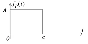
Example 2.12
Find the Laplace transform of the waveform of Figure 2.1. The subscript stands for pulse.
Figure 2.1. Waveform for Example 2.12
Solution:
We first express the given waveform as a sum of unit step functions. Then,
(2.67)
Next, from Table 2.1,
and from Table 2.2,
For this example,
and
Then, by the linearity property, the Laplace transform of the pulse of Figure 2.1 is
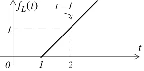
Example 2.13
Find the Laplace transform for the waveform of Figure 2.2. The subscript stands for line.
Figure 2.2. Waveform for Example 2.13
fP( )t P
A
a
t 0
fP( )t
fP( )t = A u[ 0( )t –u0(t–a)]
f t( –a)u0(t–a)⇔e–asF s( )
u0( )t ⇔1 s⁄
Au0( )t ⇔A s⁄
Au0(t–a) e–asA
s
---⇔
A u[ 0( )t –u0(t–a)] A
s ---–e–asA
s --- A
s
---(1–e–as)
= ⇔
fL( )t L
1
t
0 1
2
The Laplace Transform of Common Waveforms
Solution:
We must first derive the equation of the linear segment. This is shown in Figure 2.3. Then, we express the given waveform in terms of the unit step function.
Figure 2.3. Waveform for Example 2.13 with the equation of the linear segment
For this example,
From Table 2.1,
and from Table 2.2,
Therefore, the Laplace transform of the linear segment of Figure 2.2 is
(2.68)
Example 2.14
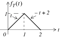
Find the Laplace transform for the triangular waveform of Figure 2.4.
Solution:
We must first derive the equations of the linear segments. These are shown in Figure 2.5. Then, we express the given waveform in terms of the unit step function.
Figure 2.4. Waveform for Example 2.14
1
t
0 1
2
fL( )t t–1
fL( )t = (t–1)u0(t–1)
f t( –a)u0(t–a)⇔e–asF s( )
tu0( )t 1
s2
----
⇔
t–1
( )u0(t–1) e–s1
s2
----⇔
fT( )t
1
t 0
1
2
Figure 2.5. Waveform for Example 2.13 with the equations of the linear segments
For this example,
and collecting like terms,
From Table 2.1,
and from Table 2.2,
Then,
or
Therefore, the Laplace transform of the triangular waveform of Figure 2.4 is
(2.69)
Example 2.15
Find the Laplace transform for the rectangular periodic waveform of Figure 2.6.
1 t
0 1
2
fT( )t
t
– +2
t
fT( )t = t u[ 0( )t –u0(t–1)]+(–t+2)[u0(t–1)–u0(t–2)]
tu0( )t –tu0(t–1)–tu0(t–1)+2u0(t–1)+tu0(t–2)–2u0(t–2)
=
fT( )t = tu0( )t –2 t( –1)u0(t–1)+(t–2)u0(t–2)
f t( –a)u0(t–a)⇔e–asF s( )
tu0( )t 1
s2
----⇔
tu0( )t –2 t( –1)u0(t–1)+(t–2)u0(t–2) 1
s2
----–2e–s1
s2
---- e–2s1
s2
----+ ⇔
tu0( )t –2 t( –1)u0(t–1)+(t–2)u0(t–2) 1
s2
----(1–2e–s+e–2s)
⇔
fT( )t 1
s2
----(1–e–s)2
⇔
The Laplace Transform of Common Waveforms
Figure 2.6. Waveform for Example 2.15
Solution:
This is a periodic waveform with period , and thus we can apply the time periodicity prop-erty
where the denominator represents the periodicity of . For this example,
Example 2.16
Find the Laplace transform for the half-rectified sine wave of Figure 2.7.
Figure 2.7. Waveform for Example 2.16
Solution:
This is a periodic waveform with period .We will apply the time periodicity property
where the denominator represents the periodicity of . For this example,
Summary
2.5 Summary
• The two-sided or bilateral Laplace Transform pair is defined as
where denotes the Laplace transform of the time function , denotes
the Inverse Laplace transform, and is a complex variable whose real part is , and imaginary
part , that is, .
• The unilateralor one-sided Laplace transform defined as
• We denote transformation from the time domain to the complex frequency domain, and vice versa, as
• The linearity property states that
• The time shifting property states that
• The frequency shifting property states that
• The scaling property states that
and in general
where the terms , and so on, represent the initial conditions.
• The differentiation in complex frequency domain property states that
andin general,
• The integration in time domain property states that
• The integration in complex frequency domain property states that
provided that the limit exists.
• The time periodicity property states that
• The initial value theorem states that
• The final value theoremstates that
Summary
• Convolution in the time domain corresponds to multiplication in the complex frequency domain, that is,
• Convolution in the complex frequency domain divided by , corresponds to multiplication in the time domain. That is,
•
The Laplace transforms of some common functions of time are shown below.
• The Laplace transforms of some common waveforms are shown below.
A
a
t 0
fP( )t
A u[ 0( )t –u0(t–a)] A
s ---–e–asA
s --- A
s
---(1–e–as)
= ⇔
1
t
0 1
2
fL( )t
t–1
( )u0(t–1) e–s1
s2
----⇔
1
t 0
1
2
fT( )t
fT( )t 1
s2
----(1–e–s)2
⇔
a
t
0 A
2a 3a
−A
fR( )t
fR( )t A
s
--- as 2
---⎝ ⎠ ⎛ ⎞
tanh
Summary
sint
1
π 2π 3π 4π
fHW( )t
fHW( )t 1
s2+1
( )(1–e–πs)
2.6 Exercises
1. Find the Laplace transform of the following time domain functions:
a.
b.
c.
d.
e.
2. Find the Laplace transform of the following time domain functions:
a.
b.
c.
d.
e.
3. Find the Laplace transform of the following time domain functions:
a.
b.
c.
d.
e. Be careful with this! Comment and skip derivation.
4. Find the Laplace transform of the following time domain functions:
a.
b.
c. 12
6u0( )t
24u0(t–12)
5tu0( )t
4t5u0( )t
j8
j5∠–90°
5e–5tu0( )t
8t7e–5tu0( )t
15δ(t–4)
t3+3t2+4t+3
( )u0( )t
3 2t( –3)δ(t–3)
3sin5t
( )u0( )t
5cos3t
( )u0( )t
2tan4t
( )u0( )t
3t(sin5t)u0( )t
2t2(cos3t)u0( )t
Exercises
d.
e.
5. Find the Laplace transform of the following time domain functions:
a.
b.
c.
d.
e.
6. Find the Laplace transform of the following time domain functions:
a.
b.
c.
d.
e.
7. Find the Laplace transform of the following time domain functions:
e.
8. Find the Laplace transform for the sawtooth waveform of Figure 2.8.
Figure 2.8. Waveform for Exercise 8.
9. Find the Laplace transform for the full rectification waveform of Figure 2.9.
Figure 2.9. Waveform for Exercise 9 e–τ
τ
---dτ t
∞
∫
fST( )t
A
a 2a t
fST( )t
3a
fFR( )t
Full Rectified Waveform sint
1
a 2a 3a 4a
Solutions to Exercises
2.7 Solutions to Exercises
1. From the definition of the Laplace transform or from Table 2.2 we get:
a. b. c. d. e.
2. From the definition of the Laplace transform or from Table 2.2 we get:
a. b. c. d. e.
3.
a. From Table 2.2 and the linearity property
b. and
c. d. e.
This answer looks suspicious because and the Laplace transform is unilateral, that is, there is one-to-one correspondence between the time domain and the complex fre-quency domain. The fallacy with this procedure is that we assumed that if and
, we cannot conclude that .
For this exercise and as we’ve learned multiplication in the time
domain corresponds to convolution in the complex frequency domain. Accordingly, we must
use the Laplace transform definition and this requires integration by parts. We
skip this analytical derivation. The interested reader may try to find the answer with the MAT-LAB code syms s t; 2*laplace(sin(4*t)/cos(4*t))
d.
e.
7. a.
but to find we must show that the limit exists. Since
this condition is satisfied and thus . From tables of integrals
. Then, and the constant of
inte-gration is evaluated from the final value theorem. Thus,
Solutions to Exercises
gration is evaluated from the final value theorem. Thus,
and using we
get
e.
, , and from tables of integrals
. Then, and the constant of integration
is evaluated from the final value theorem. Thus,
and using we
get
8.