Introduction to Orthogonal Matching Pursuit
Koredianto Usman Telkom University
Faculty of Electrical Engineering Indonesia
August 30, 2017
This tutorial is a continuation of our previous tutorial on Matching Pursuit (MP).
1 Introduction
Consider the following situation. Given
x=
−1.2 1 0
and
A =
−0.707 0.8 0 0.707 0.6 −1
Calculate y = A·x! Well this is easy. Simply
y = A·x =
−0.707 0.8 0 0.707 0.6 −1
·
−1.2 1 0
=
1.65
−0.25
.
Now the difficult part. Given
y =
1.65
−0.25
.
and
A =
−0.707 0.8 0 0.707 0.6 −1
,
In Compressive Sensing terminology, finding y from x and A is called compression. While, on the other hand, finding original x
from y and A is called reconstruction (problem). Yes, it is indeed a problem, since reconstruction is not an easy task.
As for further terminology, x is called original signal or original vector, A is called theompression matrix or sensing matrix, and
y is called compressed signal or compressed vector.
2 Basic Concept
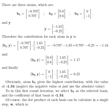
As already discussed in MP tutorial, we need to view the sensing matrix A as a collection of column vectors. That is:
A =
−0.707 0.8 0 0.707 0.6 −1
=
b1 b2 b3
,
where
b1 =
−0.707 0.707
; b2 =
0.8 0.6
; b3 =
0
−1
.
These columns are called the basis or atoms. Now, if we let
x =
x1 x2 x3
Then
A·x =
−0.707 0.707
·x1 +
0.8 0.6
·x2 +
0
−1
·x3 = y.
The last equation shows us that y is nothing but a linear combi-nation of atoms using coefficients as described in x. We know that actually x1 = −1.2, x2 = 1 and x3 = 0. In other word, looking to the last equation atom b1 contributes -1.2 to produce y, atom b2 contributes 1 to produce y, and finally, atom b3 contributes 0 to y.
3 Calculating Contribution
There are three atoms, which are:
b1 =
Therefore the contribution for each atom in y is
hb1,yi =
and finally
hb3,yi =
Obviously, atom b1 gives the highest contribution, with the value of -1.34 (neglect the negative value or just use the absolute value)
To in this first round iteration, we select b1 as the selected basis, and the coefficient of that basis is -1.34.
Of course, the dot product of each basis can be calculate in a single step, w, which is:
Figure 1 shows the illustration of basis and y.
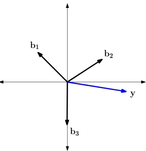
4 Calculating Residue
Now the first basis been selected, which is b1 =
−0.707 0.707
, and the
b
2b
1b
3y
Figure 1: Illustration of basis andy
from y, the residue would be:
r = y−λ1 ·b1 =
1.65
−0.25
−(−1.34)·
−0.707 0.707
=
0.7 0.7
What does this residue mean to us? Well, let see again the geometry as shown in Fig.2.
As we can see, the residue is perpendicular to the contribution of the first selected basis.
5 Repeat the iteration
After the first iteration, we get the selected basis b1. We collect this selected basis into a new Anew. That is
Anew = [b1] =
−0.707 0.707
b2
b1
b3
y
λ1 ·b1 residue r
selected basis
contribution of selected basis to y
Figure 2: Interpretation of residue
The contribution coefficient as we rewrite it as xrec is
xrec =
−1.34 0 0
.
The value -1.34 is at the first element because it is a contribution from the first basis b1.
The residue is
r =
0.7 0.7
.
Now we have to select from the rest of basis b2 and b3, which one has the highest contribution to r. In single step
w =
b2 b3T ·r =
0.8 0.6
0 −1
·
0.7 0.7
=
0.98
−0.7
So here b2 contribute better which is 0.98.
Anew =
0.707 0.6
.
Now, this step is different with MP. Here, we have to calculate the contribution of Anew to y (and not the contribution of b2 to r!).
To solve this contribution problem, we have to solve the Least Square Problem which can be easily formulated as follow:
Which λ1 dan λ2 that will fulfilled
λ1 ·
in mathematical term this formulation can be written as :
minkAnew ·λ−yk2 In our case
min
0.707 0.6
Where Anew+ is pseudo inverse of Anew, which is
Anew+ = (AnewT ·Anew)−1 ·AnewT.
Again, in our case,
Anew+ =
−0.707 0.8
0.707 0.6
+ =
−0.6062 0.8082 0.7143 0.7143
Calculating pseudo inverse is easy in Matlab, just use pinv() com-mand.
After calculating Anew+, we get
λ = Anew+ ·y =
−0.6062 0.8082 0.7143 0.7143
As we get λ, we update coefficient xrec to become
Here we put λ in the first and second position for xrec because it
corresponds to the first and second basis that have been selected. After we get Anew and λ, now we can update new the residue
r = y−Anew ·λ =
1.65
−0.25
−
−0.707 0.8
0.707 0.6
·
−1.2 1
=
0 0
.
Well, our residue is already
0 0
. So we can stop here or we can
con-tinue to the next step. (If we stop here, we can save some computation work)
6 Final iteration
This step is not necessary as the residue is already vanished. (Many OMP implemetation software requires parameter which is signal spar-sity K. This is the clue for the software that it will iterate K times. After that it will stop, no matter how much the residue left).
Our reconstructed signal is therefore :
xrec =
−1.2 1 0
Which is the same to the original signal.
7 Other example
Now we proceed with other example. Let
x =
0 3 1 2
and
A =
−0.8 0.3 1 0.4
−0.2 0.4 −0.3 −0.4
0.2 1 −0.1 0.8
Having x and A, y is calculated as
2. Since the length of basis is not one, we need to normalize them all.
ˆ
3. contribution of these normalize basis can be calculated as:
w = AˆT ·y =
−0.9428 0.268 0.9535 0.4082
−0.2357 0.3578 −0.286 −0.4082
0.2357 0.894 −0.0953 −0.8165
4. Second normalized basis ˆb2 gives the highest contribution. There-fore we take second basis and put it to Anew
Anew = bˆ2 =
5. Calculte xrec as the solution of Least Square Problem:
Lp = Anew+·y = 4.28
Since this Lp is the coefficient for basis 2, then we write
xrec =
6. Next we calculate residue
r = y−Anew ·Lp = that gives highest contribution to r.
w = AˆT·y =
−0.9428 −0.2357 0.2357
0.9535 −0.286 −0.0953
0.4082 −0.4082 −0.8165
So here, at the second position which corresponding to b3 gives the highest contribution 1.7902.
8. Add this the selected b3 (not bˆ3) in to Anew
9. Solve the Least Square Problem for Lp
Lp = Anew+·y =
We know that this Lp is for b2 and b3, therefore we write
10. Next we calculate residue
r = y−Anew·Lp =
11. Now we repeat step 2 as for the final iteration.
12. calculate highest contribution from either b1 or b4
w = ˆ
−0.9428 0.4082
−0.2357 −0.4082 0.2357 −0.8165
So here, at the second position which corresponding to b4 gives the highest contribution 0.7308.
13. And then collect this basis to already available Anew
Anew =
14. Solve the Least Square Problem for Lp
Lp = Anew+·y =
15. Next we calculate residue
16. Our iteration can be stopped here, as the residue is already zero. The reconstruction x in this case is
xrec = 0 3 1 2
which is similar to the original x.
8 Final notes
As we see in the ilustration process above, we now may notes the following facts.
• The highest contribution as we calculated from OMP is derived from normalized basis. Not from the original unnormalized basis.
• If all basis in measurement or reconstruction matrix Ahas already been normalized, the the calculation can be proceeded without normalization step.
• The contribution by each basis is done by dot product of the
residue and the normalize basis.
• In the case of MP, the reconstruction coefficient xrec is calculated
from dot product of basis and residue, while on OMP, the coeffi-cient xrec is calculated from Least Square solution of Anew to y. The solution of this Least Square Problem is actually Lp. And
Lp is directly indicates xrec with a proper positio. Anew itself is collected from already selected unnormalized basis. This process needs time. Therefore OMP is slower dan MP.
• Residue r is calculated from original y and Anew and Lp.
9 Mathematical formal algorithm for OMP
Now, after we understand previous process, we can state the following steps as OMP algorithm.
OMP algorithm
1.
10 Weakness of OMP
OMP are fast. Very fast, as compared to the convex optimization. This is an advantage of greedy algorithm. But OMP also suffers from highly coherency matrixA. What is coherency in a matrix? Coherency in matrix A simply indicates similarity between two columns in matrix
A.
Look at the following two matrix:
A1 =
0.6 0.8 1 0.8 0.6 0
and A2 =
0.6 0.61 1 0.8 0.79 0
Matrix A2 has a very high coherency, because second column is very similar to the first column. Matrix A1 has lesser coherency, because second column doesnot very similar to the first and third column. The coherency value which is denoted by µ is defined as
µ = max
i,j;i6=j|hA(:, i)·(A :, j)i|.
The value of µ is between 0 and 1. If µ is very high, then, usually OMP gives a wrong reconstruction result.
Try the following example:
x =
2 1 0
A = A2 =
0.6 0.61 1 0.8 0.79 0
Find y.
Then given A and y, using OMP, find x back! Can you get the
11 Cite this document