Parameter uncertainty analysis for simulating streamflow in a river catchment of Vietnam

Contents lists available atScienceDirect

Global Ecology and Conservation

journal homepage:www.elsevier.com/locate/gecco

Original research article

Parameter uncertainty analysis for simulating streamflow in

a river catchment of Vietnam

Dao Nguyen Khoi

a,b,∗

, Vu Thi Thom

b

a_{Faculty of Environment, University of Science, Vietnam National University Ho Chi Minh City, 227 Nguyen Van Cu, Dist.5,} Ho Chi Minh City, Viet Nam

b_{Center of Water Management and Climate Change, Vietnam National University Ho Chi Minh City, IT Park, Linh Trung Ward,} Thu Duc District, Ho Chi Minh City, Viet Nam

a r t i c l e i n f o

Article history:

Received 12 October 2015 Accepted 13 October 2015 Available online 28 October 2015

Keywords:

Srepok River Catchment SWAT model

SWAT-CUP model Uncertainty analysis

a b s t r a c t

Hydrological models play vital roles in management of water resources. However, the cali-bration of the hydrological models is a large challenge because of the uncertainty involved in the large number of parameters. In this study, four uncertainty analysis methods, in-cluding Generalized Likelihood Uncertainty Estimation (GLUE), Parameter Solution (Para-Sol), Particle Swarm Optimization (PSO), and Sequential Uncertainty Fitting (SUFI-2), were employed to perform parameter uncertainty analysis of streamflow simulation in the Sre-pok River Catchment by using the Soil and Water Assessment Tool (SWAT) model. The four methods were compared in terms of the model prediction uncertainty, the model perfor-mance, and the computational efficiency. The results showed that the SUFI-2 method has the advantages in the model calibration and uncertainty analysis. This technique could be run with the smallest of simulation runs to achieve good prediction uncertainty bands and model performance. This technique could be run with the smallest of simulation runs to achieve good prediction uncertainty bands and model performance.

©2015 The Authors. Published by Elsevier B.V. This is an open access article under the CC BY-NC-ND license (http://creativecommons.org/licenses/by-nc-nd/4.0/).

1. Introduction

Hydrological model is a useful tool in managing and planning water resources. In recent years, a large number of hydrological models have been developed and can be classified into lumped and distributed models. The distributed hydrological model is preferable, since it can realistically represent the spatial variability of catchment characteristics (Oeurng et al., 2011). In recent years, many such hydrological models have been developed such as AGNPS (Agricultural Non-Point Source) (Young et al., 1989), HSPF (Hydrologic Simulation Program—Fortran) (Bicknell et al., 2000), MIKE SHE (Refsgaard and Storm, 1995), and SWAT (Soil and Water Assessment Tool) (Arnold et al., 1998). Among these models, the SWAT is one of the choices because it is widely used to assess hydrology in small and large catchments around the world (see SWAT Literature database:http://www.card.iastate.edu/swat_articles/). The ability of the hydrological model to accurately simulate the hydrological process is assessed through a careful calibration and uncertainty analysis. Calibration of hydrological models is a challenging task because of uncertainties in hydrological modeling (Yang et al., 2008). According to

Xue et al.(2014), the main sources of uncertainties are model inputs associated with measurement errors, from model structures due to assumption and simplification, and from model parameters related to approximations. Among these

∗_{Corresponding author at: Faculty of Environment, University of Science, Vietnam National University Ho Chi Minh City, 227 Nguyen Van Cu, Dist.5, Ho}

Chi Minh City, Viet Nam.

E-mail address:dnkhoi86@gmail.com(D.N. Khoi).

http://dx.doi.org/10.1016/j.gecco.2015.10.007

sources of uncertainty, the parameter uncertainty is inevitable but it is easy to control by using a suitable calibration method (Wu and Chen,2015).

To account for that uncertainty, a number of uncertainty analysis techniques have been developed and applied to many hydrological studies. For example,Shen et al.(2012) used Generalized Likelihood Uncertainty Estimation (GLUE) method coupled with the SWAT model to estimate the parameter uncertainty of the streamflow and sediment simulation in the Daning River Watershed, China;Rostamian et al.(2008) used Sequential Uncertainty Fitting (SUFI-2) to perform model calibration and uncertainty analysis in the Beheshtabad and Vanak river catchments in the central Iran;van Griensven et al.

(2008) applied Parameter Solution (ParaSol) method to estimate parameter uncertainty in the SWAT model of Honey Creek, a tributary of the Sandusky catchment in Ohio, USA; andSamadi and Meadows(2014) used Particle Swarm Optimization (PSO) method to investigate uncertainty analysis in the SWAT hydrological model at the Waccamaw River Catchment, USA. However, a few studies have been reported on comparison of different uncertainty analysis techniques. For instance,Wu and Chen(2015) evaluated uncertainty estimates in distributed hydrological modeling for the Wenjing River watershed in China by GLUE, SUFI-2, and ParaSol methods, and they indicated that the SUFI-2 method is able to provide more reasonable simulated results than the other two methods. Another similar study in a river basin of eastern India conducted byUniyal et al.(2015) reported that both SUFI-2 and GLUE are the promising techniques for uncertainty analysis of modeling results and there is a need to conduct such types of studies in different catchments under varying agro-climatic conditions for assessing their generic capability.

From the above review of literature, it is apparent that the generality of using different uncertainty analysis techniques needs to be verified with more applications to different regions. In addition, the studies on uncertainty analysis of hydrological modeling in Vietnam has not been conducted yet. The objective of this paper is to apply the four uncertainty analysis techniques (i.e., SUFI-2, GLUE, ParaSol, and PSO) to perform parameter uncertainty analysis for streamflow simulation. A case study was conducted in the Srepok River Catchment in the Central Highlands of Vietnam, by using the SWAT distributed hydrological model. The results of this study provide a scientific reference based on uncertainty analysis to decision-makers in order to promote water resources planning efforts.

2. Study area

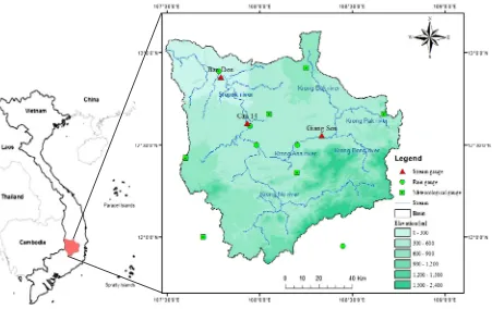
The Srepok River Catchment, a sub-basin of the Mekong River Basin, is located in the Central Highlands of Vietnam, and lies between latitudes 11°₄₅′′_–13°15′′_{N and longitudes 107°15}′′_{–109°E (Fig. 1). The Srepok River is formed by two}

main tributaries: the Krong No and Krong Ana rivers. The total area of this catchment is approximately 12,000 km2with the population of 2.2 million (2009). The average altitude of the watershed varies from 100 m in the northwest to 2400 m in the southeast. The climate in the area is very humid (78%–83% annual average humidity) with annual rainfall varying from 1700 mm to 2300 mm and features a distinct wet and dry seasons. The wet season lasts from May to October (with peak floods often in September and October) and accounts for over 75%–95% of the annual precipitation. The mean annual temperature is 23°C. In this catchment, there are two dominant soils: grey soil and red-brown basaltic soil. These soils are highly fertile and very consistent with agricultural development. Agriculture is the main economic activity in this catchment of which coffee and rubber production are predominant.

3. Methodology

3.1. SWAT hydrological model

The SWAT model is a physically based distributed model designed to predict the impact of land management practices on water, sediment, and agricultural chemical yields in large complex watersheds with varying soil, land-use, and management conditions over long periods of time (Neitsch et al., 2011). With this model, a catchment is divided into a number of sub-watersheds or sub-basins. Sub-basins are further partitioned into hydrological response units (HRUs) based on soil types, land-use types, and slope classes that allow a high level of spatial detail simulation. The model predicts the hydrology at each HRU using the water balance equation as follows:

SWt

=

SW0

+

t



i=1



Rday

−

Qsurf

−

Ea

−

w

seep

−

Qgw



(1)

whereSWt is the final soil water content (mm H2O),SW0is the initial soil water content on dayi(mm H2O),tis the time (days),Rdayis the amount of precipitation on dayi(mm H2O),Qsurfis the amount of surface runoff on dayi(mm H2O),Eais

the amount of evapotranspiration on dayi(mm H2O),

w

seepis the amount of water entering the vadose zone from the soil

profile on dayi(mm H2O), andQgwis the amount water return flow on dayi(mm H2O). A detail description of the different model components can be found in the SWAT Theoretical Documentation (Neitsch et al., 2011).

Fig. 1. Location map of the Srepok River Catchment. (For interpretation of the references to color in this figure legend, the reader is referred to the web version of this article.)

Table 1

Data sources used in the initial setup of the SWAT model for the Srepok River Catchment.

Data type Data description Scale Data sources

Topography Elevation 30 m Aster GDEM

Land-use Land-use classification such as agricultural land, forest, and urban 1 km MRC

Soil Soil types and physical properties 10 km FAO

Meteorology Daily precipitation, minimum and maximum temperature Daily Hydro-Meteorological Data Center (HMDC)

The model set-up consists of four steps: (1) data preparation, (2) sub-basin discretization, (3) HRU definition, (4) calibration and uncertainty analysis. The SWAT coupled with ArcGIS as the ArcSWAT is used for watershed delineation and other purposes. The ArcGIS 10.1 and ArcSWAT 2012 were used in this study. The calibration and uncertainty analysis were done using four different algorithms, i.e. SUFI-2, GLUE, ParaSol, and PSO, which are implemented in the SWAT-CUP 2012 (Abbaspour, 2014).

The Nash-Sutcliffe efficiency (NSE), percent bias (PBIAS), and ratio of the RMSE to the standard deviation of measured data (RSR) were used as statistical indices to assess the goodness of fit of the model. According toMoriasi et al.(2007), the model performance for flow simulation can be judged as ‘‘satisfactory’’ if 0

.

6

<

RSR

≤

0

.

7

,

0

.

5

<

NSE

≤

0

.

7, and

±

15%

≤

PBIAS

<

±

25%; ‘‘good’’ if 0

.

5

<

RSR

≤

0

.

6

,

0

.

7

<

NSE

≤

0

.

8, and

±

10%

≤

PBIAS

<

±

15%; and ‘‘very good’’ if 0

.

0

≤

RSR

≤

0

.

0

,

0

.

8

<

NSE

≤

1

.

0, and PBIAS

≤ ±

10%.

3.2. Uncertainty analysis methods

3.2.1. GLUE

The GLUE was introduced partly to allow for possible non-uniqueness of parameter sets during the estimation of model parameters in over-parameterized models. It is an uncertainty analysis inspired by importance sampling or regional sensitivity analysis (Hornberger and Spear, 1981). Similar to SUFI-2, GLUE accounts for all sources of uncertainty because the likelihood measure value is associated with a parameter set and reflects all these sources of error and any effects of the co-variation of parameters values on model performance implicitly (Beven and Freer, 2001). The three major steps of the GLUE method are shown below (Yang et al.,2008;Abbaspour,2014):

Step 1: After the definition of the ‘‘generalized likelihood measures’’L

(θ )

, a large number of parameter sets are randomly sampled from the prior distribution and each parameter set is assessed as either ‘‘behavioral’’ or ‘‘non-behavioral’’ through a comparison of the ‘‘likelihood measure’’ with the given threshold value.

Step 2: Each behavioral parameter is given a ‘‘likelihood weight’’ according to:

w

i

=

L

(θ

i

)

N



k=1

L

(θ

k

)

(2)

whereNis the number of behavioral parameter sets.

Step 3: The prediction uncertainty is described as prediction quantiles from the cumulative distribution realized from the weighted behavioral parameter sets. In this study, the NSE are selected as the model efficiency measurement.

3.2.2. ParaSol

The ParaSol method aggregates objective function (OF’s) into a global optimization criterion (GOC), minimizes these OF’s or a GOC using the Shuffle Complex Evolution algorithm (SCE-UA) and performs uncertainty analysis with a choice between two statistical concepts. The SCE-UA algorithm is a global search algorithm for the minimization of a single function for up to 16 parameters (Duan et al., 1992). The procedure of ParaSol is as follows (Yang et al.,2008;Abbaspour,2014):

Step 1: After the optimization of the modified SCE-UA (the randomness of the algorithm SCE-UA is increased to improve the coverage of the parameter space), the simulations performed are divided into ‘good’ simulations and ‘not good’ simulations by a threshold value of the objective function as in the GLUE method. The objective function used in the ParaSol method is the sum of the squares of the residuals (SSQ):

SSQ

=

n



ti=1



yM_t

i

(θ )

−

yti



2

.

(3)

The relationship between NSE and SSQ is

NSE

=

1

−

_n 1



ti=1



yti

− ¯

y



2

SSQ (4)

where



n

ti



yti

− ¯

y



2

is a fixed value for give observations. To compare with SUFI-2 and GLUE, all objective function values of ParaSol are converted to NSE.

Step 2: The prediction uncertainty is hence constructed equally from the ‘good’ simulations.

3.2.3. PSO

Particle swarm optimization (PSO) is a population based stochastic optimization technique developed byEberhart and Kennedy(1995). PSO has a lot of similarities with evolutionary computation techniques such as Genetic Algorithms (GA). Compared to GA, PSO is easy to implement and there are few parameters to adjust.

PSO is initialized with a group of random particles (solutions) and then searches for optima by updating generations. In every iteration, each particle is updated by following two ‘‘best’’ values. The first one is the best solution which has achieved so far. This values is calledpbest. Another ‘‘best’’ value that is tracked by the particle swarm optimizer is the best value, obtained so far by any particle in the population. This best value is calledgbest. When a particle takes part of the population as its topological neighbors, the best value is a local best and it is calledlbest.

After finding the two best values, the particles updates its velocity and positions with the following equations.

v[] =

v[] +

b1

×

rand

()

×

(

pbest

[] −

present

[])

+

b2

×

rand

()

×

(

gbest

[] −

present

[])

(5)

present

[] =

present

[] +

v[]

(6)

Table 2

Selected parameters of the SWAT model for uncertainty analysis.

Parameters Description Range

r_CN2 Initial SCS CNII value −0.30, to 0.30

v_ESCO Soil evaporation compensation factor 0, to 1.00

v_GWQMN Threshold water depth in the shallow aquifer for flow −1000, to 2500

v_ALPHA_BF Baseflow alpha factor 0, to 1.00

r_SOL_Z Soil depth −0.20, to 0.20

r_SOL_AWC Available water capacity −0.20, to 0.20

v_CH_K2 Channel effective hydraulic conductivity −100.0, to 100.0

v_GW_REVAP Groundwater ‘revap’ coefficient 0, to 0.20

v_CH_N2 Manning’s value for main channel 0, to 0.30

r_SOL_K Saturated hydraulic conductivity −0.20, to 0.20

v_means the existing parameter value is to be replaced by the given value. r_means the existing parameter value is multiplied by (1+a given value).

3.2.4. SUFI-2

The SUFI-2 method is based on a Bayesian framework, and it determines uncertainties through the sequential and fitting process. In SUFI-2, parameter uncertainty accounts for all sources of uncertainty, such as model input, model structure, model parameters, and measured data. SUFI-2 executes a combined optimization and uncertainty analysis using a global search method and deal with plenty of parameters through Latin Hypercube sampling (Abbaspour, 2014). The procedure of the SUFI-2 algorithm is as follows (Yang et al.,2008;Abbaspour,2014):

Step 1: In the first step, the objective function g(b) and the initial uncertainty ranges

[

bj,abs_mean

,

bj,abs_ max

]

for the parameters are defined. In this study, we chose the Nash-Sutcliffe efficiency (NSE) as the objective function.

wherebjis thejth parameter;j

=

1

, . . . ,

m; andmis the number of parameters to be estimated.

Step 2: The Latin Hypercube sampling is carried out in the hypercube

[

bmin

,

bmax

]

(initially set to

[

bj,abs_mean

,

bj,abs_ max

]

), the corresponding objective functions are assessed, and the sensitivity matrixJand the parameter covariance matrixCare calculated as follows:

Jij

=

1gi

1bj

i

=

1

, . . . ,

C₂n

;

j

=

1

, . . . ,

m (7)

C

=

s2_g



JTJ



−1

(8)

wheres2

gis all combinations of two simulations,s2gis the variance of the objective function values resulting from thenruns.

Step 3: The 95PPU is calculated. It has two indices, i.e. thep-factor andr-factor. Ther-factor is estimated:

r-factor

=

¯

dX

σ

X

(9)

where

σ

X is the standard deviation of the measured variableX; andd

¯

is the average distance between upper and lower

boundary of 95PPU, is calculated:

¯

dX

=

1 k

k



l=1

(

XU

−

XL

)

l (10)

wherelis a counter;kis the number of observed data points; andQL(2.5th) andQU(97.5th) is the lower and upper boundary

of the 95PPU.

Step 4: Because parameter uncertainties are initially large, the value ofd

¯

tends to be quite large during the first sampling round. Therefore, further sampling rounds are needed with updated parameter ranges.

4. Results and discussion

4.1. Uncertainty analysis

The SWAT hydrological parameters used for calibration and uncertainty analysis of streamflow simulation were selected by referring the relevant study in the Be River Catchment (Khoi and Suetsugi, 2012). The selected parameters for the flow simulation were CN2, ESCO, GWQMN, ALPHA_BF, SOL_Z, SOL_AWC, CH_K2, GW_REVAP, and SOL_K. These sensitive parameters were identified by using Latin Hypercube One-factor-At-a-Time (LH-OAT) technique. Furthermore,Uniyal et al.

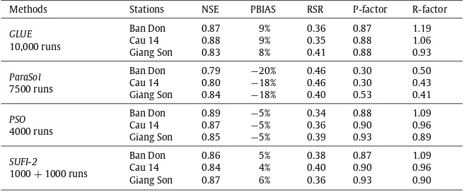
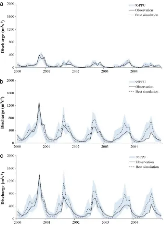
Fig. 2. Simulated and observed daily flow at (a) Giang Son station, (b) Cau 14 station, and (c) Ban Don station by using the GLUE method.

4.1.1. GLUE method

The GLUE method is relatively simple and widely used in hydrology. According toYang et al.(2008), they performed the GLUE simulations with four sample sizes of 1000, 5000, 10,000, and 20,000 runs, and the result showed that the sample size of 10,000 runs is best. Therefore, 10,000 simulation runs were conducted for the uncertainty analysis in this study. And, the threshold value is selected to be 0.70, i.e., the simulations with the NSE values larger than 0.70 are behavioral otherwise non-behavioral.Fig. 2shows the 95PPU for the model results derived by the GLUE method. The simulation results of the Giang Son, Cau 14, and Ban Don stations are relatively good, which 83%–88% observations equal with 95PPU during the calibration period, and P-factor, NSE, PBIAS, and RSR values are within the criteria suggested byMoriasi et al.(2007), namely the fits between the simulated and observed values are well at all stations (seeTable 3).

4.1.2. ParaSol method

Table 3

The statistic summary of the results of four uncertainty analysis techniques.

Methods Stations NSE PBIAS RSR P-factor R-factor

GLUE

10,000 runs

Ban Don 0.87 9% 0.36 0.87 1.19

Cau 14 0.88 9% 0.35 0.88 1.06

Giang Son 0.83 8% 0.41 0.88 0.93

ParaSol

7500 runs

Ban Don 0.79 −20% 0.46 0.30 0.50

Cau 14 0.80 −18% 0.46 0.30 0.43

Giang Son 0.84 −18% 0.40 0.53 0.41

PSO

4000 runs

Ban Don 0.89 −5% 0.34 0.88 1.09

Cau 14 0.87 −5% 0.36 0.90 0.96

Giang Son 0.85 −5% 0.39 0.93 0.89

SUFI-2

1000+1000 runs

Ban Don 0.86 5% 0.38 0.87 1.09

Cau 14 0.84 4% 0.40 0.90 0.96

Giang Son 0.87 6% 0.36 0.93 0.90

method failed to derive the reasonable prediction uncertainty although the best simulation matches the observation quite well with NSE, PBIAS, and RSR equal to 0.84, 0.80, and 0.79,

−

18%,

−

18%, and

−

20%, and 0.40, 0.46, and 0.46, at the Giang Son, Cau 14, and Ban Don stations, respectively. This is because the ParaSol method does not consider the uncertainties in the model structure (spatial scaling, mathematical equations) and model input data (rainfall, temperature, etc.) (van Griensven and Meixner, 2007). Another reason is related to the statistical assumption of ParaSol, which violates independent and normally distributed errors (Yang et al.,2008;Zhang et al.,2015).

4.1.3. PSO method

About the PSO method, 4000 simulation runs were conducted for uncertainty analysis (Yang et al.,2008;Zhang et al.,

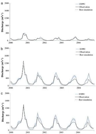
2015). For a better comparison, the NSE value of 0.7 was selected as the objective function. The initial parameter ranges used in the PSO method are the same as those adopted in the GLUE and ParaSol methods.Table 3shows the statistic summary of the simulation results, such as NSE, PBIAS, RSR, P-factor, and R-factor.Fig. 4presents the hydrograph of simulated and observed values obtained by the ParaSol method, which describes the 95PPU. As shown inFig. 4, the 95PPU region from PSO is narrower than that of the GLUE method, which is corresponding to the values of the R-factor (seeTable 3). The NSE values are 0.85, 0.87, and 0.89; the PBIAS values are

−

5%, and the RSR values are 0.39, 0.36, and 0.34 for the Giang Son, Cau 14, and Ban Don stations, respectively. The best simulation of the PSO method is quite similar to the results from the GLUE method (seeTable 3).

4.1.4. SUFI-2 method

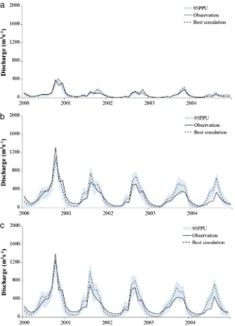
SUFI-2 is easy to implement. Because the sampling method in SUFI-2 is Latin Hypercube sampling method, it can reduce the sampling sizes comparing to the Monte Carlo random sampling method (Wu and Chen,2015). Normally, the sample size for one iteration could be set in the range of 500–1000 runs. In this study, two iterations with 1000 model runs in each iteration were conducted for uncertainty analysis.Fig. 5shows the 95PPU for the model results derived by the SUFI-2 method from the second iteration. It is shown that 93% measurements at the Giang Son station, 90% measurements at the Cau 14 station, and 87% measurements at the Ban Don station are bracketed by the 95PPU, indicating SUFI-2 is capable of capturing the observations. The 95PPU region from SUFI-2 is similar to that of the PSO method, which corresponding to that values of R-factor shown inTable 3. In addition, the values of NSE, PBIAS, and RSR of the best simulation are quite similar to the results from the GLUE and PSO methods for all stations (seeTable 3).

4.2. Comparison

For comparison of different uncertainty methods, including the GLUE, ParaSol, PSO, and SUFI-2 methods, it is conducted in three aspects: the model performance, the model prediction uncertainty, and the model computational efficiency.

Table 3presents the statistic summary of the uncertainty analysis results of the four methods. In terms of the model performance, all the four methods obtained similarly good results based on the performance criteria given byMoriasi et al.

Fig. 3. Simulated and observed daily flow at (a) Giang Son station, (b) Cau 14 station, and (c) Ban Don station by using the ParaSol method.

About the prediction uncertainty, the ParaSol method gave too narrow prediction uncertainty bands which are hardly distinguishable from its best prediction. This may have resulted from violation of the statistical assumption of independent and normally distributed residuals. According to the simulation results shown inTable 3, the R-factors for the streamflow by using GLUE are larger than those by using PSO and SUFI-2. This shows that the prediction uncertainty range from the GLUE method is wider than that from the PSO and SUFI-2 methods. This is likely attributed to the larger number of simulation runs (10,000 runs) in the GLUE method compared to those in the other two methods (4000 runs for PSO and 2000 runs for SUFI-2).

Fig. 4. Simulated and observed daily flow at (a) Giang Son station, (b) Cau 14 station, and (c) Ban Don station by using the PSO method.

intensive computations (10,000 runs) because the Monte Carlo sampling method was applied. Generally, the computational efficiency of the SUFI-2 method is higher than that from the other three methods.

Fig. 5. Simulated and observed daily flow at (a) Giang Son station, (b) Cau 14 station, and (c) Ban Don station by using the SUFI-2 method.

5. Conclusion

Model uncertainty analysis is one of the important research contents of hydrological models. In this study, four uncertainty analysis methods, including GLUE, ParaSol, PSO, and SUFI-2, were studied through the SWAT hydrological model in order to examine their performance and capability in quantifying parameter uncertainties. A case study was conducted in the Srepok River Catchment in the Central Highlands of Vietnam. The following conclusions could be summarized from this study:

– The SWAT model could simulate satisfactorily the streamflow for the study area with the satisfactory values of NSE, PBIAS, and RSR. The results indicated that the SWAT model is a useful tool for simulating hydrological processes in the Srepok River Catchment.

This study suggested that the SUFI-2 method is a useful tool in calibration and uncertainty analysis to support studies on impact of climate change and human activities on water resources in sub-tropical and tropical areas as well as in Vietnam by using hydrological model with more reasonable and accurate predictions. Although this study provided interesting findings from the comparison of the four uncertainty analysis methods, the generality of such findings still needs to be verified with more applications to different study areas in the future studies.

Acknowledgment

This research is funded by Vietnam National Foundation for Science and Technology Development (NAFOSTED) under grant number ‘‘105.06-2013.09’’.

References

Abbaspour, K.C., 2014. SWAT-CUP 2012: SWAT Calibration and Uncertainty Programs—A User Manual. Swiss Federal Institute of Aquatic Science and Technology.

Arnold, J.G., Srinivasan, P., Muttiah, R.S., Williams, J.R.,1998. Large area hydrologic modeling and assessment, Part I: Model development. J. Am. Water Resour. Assoc. 34, 73–89.

Beven, K., Freer, J.,2001. Equifinality, data assimilation and uncertainty estimation in mechanistic modeling of complex environmental system using the GLUE methodology. J. Hydrol. 249 (1–4), 11–29.

Bicknell, B.R., Imhpff, J.C., Kittle, J.L., Jobes, T.H., Donigian, A.S.,2000. Hydrological Simulation Program—Fortran (HSPF); User’s Manual for Release 12. USEPA, Athens, Ga..

Duan, Q.Y., Sorooshian, S., Gupta, V., 1992. Effective and efficient global optimization for conceptual rainfall-runoff models. Water Resour. Res. 28 (4), 1015–1031.http://dx.doi.org/10.1029/91WR02985.

Eberhart, R.C., Kennedy, J.A.,1995. A new optimizer using particle swarm theory. In: Proceedings of the Sixth International Symposium on Micro Machine and Human Science. IEEE Service Center, Piscataway, NJ, Nagoya, Japan.

Hornberger, G.M., Spear, R.C.,1981. An approach to the preliminary analysis of environmental system. J. Environ. Manag. 12 (1), 7–18.

Khoi, D.N., Suetsugi, T.,2012. Hydrologic response to climate change: a case study for the Be River Catchment, Vietnam. J. Water Clim. Change 3 (3), 207–224.

Moriasi, D.N., Arnold, J.G., Van Liew, M.W., Bingner, R.L., Harmel, R.D., Veith, T.L.,2007. Model evaluation guidelines for systematic quantification of accuracy in watershed simulations. Trans. ASABE 50, 885–900.

Neitsch, A.L., Arnold, J.G., Kiniry, J.R., Williams, J.R.,2011. Soil and water assessment tool theoretical documentation version 2009. Texas Water Resources Institute Technical Report No. 406. Texas A&M University, Texas.

Oeurng, C., Sauvage, S., Sanchez-Perez, J.M.,2011. Assessment of hydrology, sediment and particulate organic carbon yield in a large agricultural catchment using the SWAT model. J. Hydrol. 401, 145–153.

Refsgaard, J.C., Storm, B.,1995. MIKE SHE. In: Singh, V.P. (Ed.), Computer Models of Watershed Hydrology. Water Resources Publications, Colorado, USA, pp. 809–846. (Chapter 22).

Rostamian, R., Jaleh, A., Afyuni, M., Mousavi, S.F., Heidarpour, M., Jalalian, A., Abbaspour, K.C.,2008. Application of a SWAT model for estimating runoff and sediment in two mountainous basins in central Iran. Hydrol. Sci. J. 53 (5), 977–988.

Samadi, S., Meadows, M.E., 2014. Examining the robustness of the SWAT distributed model using PSO and GLUE uncertainty frameworks. In: Proceedings of the 2014 South Carolina Water Resources Conference, Columbia, USA.

Shen, Z.Y., Chen, L., Chen, T.,2012. Analysis of parameter uncertainty in hydrological and sediment modeling using GLUE method: a case study of SWAT model applied to Three Gorges Reservoir Region, China. Hydrol. Earth Syst. Sci. 16, 121–132.

Uniyal, B., Jha, M.K., Verma, A.K., 2015. Parameter identification and uncertainty analysis for simulating streamflow in a river basin of Eastern India. Hydrol. Process. 29 (17), 3744–3766.http://dx.doi.org/10.1002/hyp.10446.

van Griensven, A., Meixner, T., 2007. A global and efficient multi-objective auto-calibration and uncertainty estimation method for water quality catchment models. J. Hydroinform. 9 (4), 277–291.http://dx.doi.org/10.2166/hydro.2007.104.

van Griensven, A., Meixner, T., Srinivasan, R., Grunwald, S., 2008. Fit-for-purpose analysis of uncertainty using split-sampling evaluations. Hydrol. Sci. J. 53 (5), 1090–1103.http://dx.doi.org/10.1623/hysj.53.5.1090.

Wu, H., Chen, B., 2015. Evaluating uncertainty estimates in distributed hydrological modeling for the Wenjing River watershed in China by GLUE, SUFI-2, and ParaSol methods. Ecol. Eng. 76, 110–121.http://dx.doi.org/10.1016/j.ecoleng.2014.05.014.

Xue, C., Chen, B., Wu, H.,2014. Parameter uncertainty analysis of surface flow and sediment yield in the Huolin Basin, China. J. Hydrol. Eng. 19 (6), 1224–1236.

Yang, J., Reichert, P., Abbaspour, K.C., Xia, J., Yang, H.,2008. Comparing uncertainty analysis techniques for a SWAT application to the Chaohe Basin in China. J. Hydrol. 358, 1–23.

Young, R.A., Onstad, C.A., Bosch, D.D.,1989. AGNPS: a nonpoint source pollution model for evaluating agricultural watersheds. J. Soil Water Conserv. 44 (2), 168–173.