2017943790 © 2017 The Cylance Data Science Team
All rights reserved. No part of this publication may be reproduced, stored in a retrieval system, or transmitted in any form or by any means electronic, mechanical, photocopying, recording or otherwise, without the prior written permission of the publisher.
Published by
The Cylance Data Science Team.
Introduction to artificial intelligence for security professionals / The Cylance Data Science Team. – Irvine, CA: The Cylance Press, 2017.
p. ; cm.
Summary: Introducing information security professionals to the world of artificial intelligence and machine learning through explanation and examples.
ISBN13: 978-0-9980169-2-4
1. Artificial intelligence. 2. International security. I. Title.
FIRST EDITION
Project coordination by Jenkins Group, Inc. www.BookPublishing.com
Interior design by Brooke Camfield
Contents
Front Cover Title Page
Copyright Page Contents
Foreword Introduction
Artificial Intelligence: The Way Forward in Information Security
1 Clustering
Using the K-Means and DBSCAN Algorithms
2 Classification
Using the Logistic Regression and Decision Tree Algorithms 3 Probability
Foreword
by Stuart McClure
My first exposure to applying
a science to computers came at the University of Colorado, Boulder, where, from 1987-1991, I studied Psychology, Philosophy, and Computer Science Applications. As part of the Computer Science program, we studied Statistics and how to program a computer to do what we as humans wanted them to do. I remember the pure euphoria of controlling the machine with programming languages, and I was in love.In those computer science classes we were exposed to Alan Turing and the quintessential “Turing Test.” The test is simple: Ask two “people” (one being a computer) a set of written questions, and use the responses to them to make a determination. If the computer is indistinguishable from the human, then it has “passed” the test. This concept intrigued me. Could a computer be just as natural as a human in its answers, actions, and thoughts? I always thought, Why not?
Flash forward to 2010, two years after rejoining a tier 1 antivirus company. I was put on the road helping to explain our roadmap and vision for the future. Unfortunately, every conversation was the same one I had been having for over twenty years: We need to get faster at detecting malware and cyberattacks. Faster, we kept saying. So instead of monthly signature updates, we would strive for weekly updates. And instead of weekly we would fantasize about daily signature updates. But despite millions of dollars driving toward faster, we realized that there is no such thing. The bad guys will always be faster. So what if we could leap frog them? What if we could actually predict what they would do before they did it?
what was bad and good. So when I finally left that antivirus company, I asked myself, “Why couldn’t I train a computer to think like me—just like a security professional who knows what is bad and good? Rather than rely on humans to build signatures of the past, couldn’t we learn from the past so well that we could eliminate the need for signatures, finally predicting attacks and preventing them in real time?”
And so Cylance was born.
My Chief Scientist, Ryan Permeh, and I set off on this crazy and formidable journey to completely usurp the powers that be and rock the boat of the establishment—to apply math and science into a field that had largely failed to adopt it in any meaningful way. So with the outstanding and brilliant Cylance Data Science team, we achieved our goal: protect every computer, user, and thing under the sun with artificial intelligence to predict and prevent cyberattacks.
So while many books have been written about artificial intelligence and machine learning over the years, very few have offered a down to earth and practical guide from a purely cybersecurity perspective. What the Cylance Data Science Team offers in these pages is the very real-world, practical, and approachable instruction of how anyone in cybersecurity can apply machine learning to the problems they struggle with every day: hackers.
Introduction
Artificial Intelligence: The Way
Forward in Information Security
Artificial Intelligence (AI) technologies are
rapidly moving beyond the realms of academia and speculative fiction to enter the commercial mainstream. Innovative products such as Apple’s Siri® digital assistant and the Google search engine, among others, are utilizing AI to transform how we access and utilize information online. According to a December 2016 report by the Office of the President:Advances in Artificial Intelligence (AI) technology and related fields have opened up new markets and new opportunities for progress in critical areas such as health, education, energy, economic inclusion, social welfare, and the environment.1
AI has also become strategically important to national defense and securing our critical financial, energy, intelligence, and communications infrastructures against state-sponsored cyber-attacks. According to an October 2016 report2
issued by the federal government’s National Science and Technology Council Committee on Technology (NSTCC):
AI has important applications in cybersecurity, and is expected to play an increasing role for both defensive and offensive cyber measures. . . . Using AI may help maintain the rapid response required to detect and react to the landscape of evolving threats.
Intelligence Research and Development Strategic Plan3 to guide
federally-funded research and development.
Like every important new technology, AI has occasioned both excitement and apprehension among industry experts and the popular media. We read about computers that beat Chess and Go masters, about the imminent superiority of self-driving cars, and about concerns by some ethicists that machines could one day take over and make humans obsolete. We believe that some of these fears are over-stated and that AI will play a positive role in our lives as long AI research and development is guided by sound ethical principles that ensure the systems we build now and in the future are fully transparent and accountable to humans.
In the near-term however, we think it’s important for security professionals to gain a practical understanding about what AI is, what it can do, and why it’s becoming increasingly important to our careers and the ways we approach real-world security problems. It’s this conviction that motivated us to write
Introduction to Artificial Intelligence for Security Professionals.
You can learn more about the clustering, classification, and probabilistic modeling approaches described in this book from numerous websites, as well as other methods, such as generative models and reinforcement learning. Readers who are technically-inclined may also wish to educate themselves about the mathematical principles and operations on which these methods are based. We intentionally excluded such material in order to make this book a suitable starting point for readers who are new to the AI field. For a list of recommended supplemental materials, visit https://www.cylance.com/intro-to-ai.
AI: Perception Vs. Reality
The field of AI actually encompasses three distinct areas of research:
Artificial Superintelligence (ASI) is the kind popularized in speculative fiction and in movies such as The Matrix. The goal of ASI research is to produce computers that are superior to humans in virtually every way, possessing what author and analyst William Bryk referred to as “perfect memory and unlimited analytical power.”4
Artificial General Intelligence (AGI) refers to a machine that’s as intelligent as a human and equally capable of solving the broad range of problems that require learning and reasoning. One of the classic tests of AGI is the ability to pass what has come to be known as “The Turing Test,”5 in which a human evaluator reads a text-based conversation
occurring remotely between two unseen entities, one known to be a human and the other a machine. To pass the test, the AGI system’s side of the conversation must be indistinguishable by the evaluator from that of the human.
Most experts agree that we’re decades away from achieving AGI and some maintain that ASI may ultimately prove unattainable. According to the October 2016 NSTC report,6 “It is very unlikely that machines will
exhibit broadly-applicable intelligence comparable to or exceeding that of humans in the next 20 years.”
Artificial Narrow Intelligence (ANI) exploits a computer’s superior ability to process vast quantities of data and detect patterns and relationships that would otherwise be difficult or impossible for a human to detect. Such data-centric systems are capable of outperforming humans only on specific tasks, such as playing chess or detecting anomalies in network traffic that might merit further analysis by a threat hunter or forensic team. These are the kinds of approaches we’ll be focusing on exclusively in the pages to come.
applying algorithms to data. Often, the terms AI and ML are used interchangeably. In this book, however, we’ll be focusing exclusively on methods that fall within the machine learning space.
Machine Learning in the Security Domain
In order to pursue well-defined goals that maximize productivity, organizations invest in their system, information, network, and human assets. Consequently, it’s neither practical nor desirable to simply close off every possible attack vector. Nor can we prevent incursions by focusing exclusively on the value or properties of the assets we seek to protect. Instead, we must consider the context
in which these assets are being accessed and utilized. With respect to an attack on a website, for example, it’s the context of the connections that matters, not the fact that the attacker is targeting a particular website asset or type of functionality.
Context is critical in the security domain. Fortunately, the security domain generates huge quantities of data from logs, network sensors, and endpoint agents, as well as from distributed directory and human resource systems that indicate which user activities are permissible and which are not. Collectively, this mass of data can provide the contextual clues we need to identify and ameliorate threats, but only if we have tools capable of teasing them out. This is precisely the kind of processing in which ML excels.
The Future of Machine Learning
As ML proliferates across the security landscape, it’s already raising the bar for attackers. It’s getting harder to penetrate systems today than it was even a few years ago. In response, attackers are likely to adopt ML techniques in order to find new ways through. In turn, security professionals will have to utilize ML defensively to protect network and information assets.
We can glean a hint of what’s to come from the March 2016 match between professional Go player Lee Sedol an eighteen-time world Go champion, and AlphaGo a computer program developed at DeepMind, an AI lab based in London that has since been acquired by Google. In the second game, AlphaGo made a move that no one had ever seen before. The commentators and experts observing the match were flummoxed. Sedol himself was so stunned it took him nearly fifteen minutes to respond. AlphaGo would go on to win the best-of-five game series.
In many ways, the security postures of attack and defense are similar to the thrust and parry of complex games like Go and Chess. With ML in the mix, completely new and unexpected threats are sure to emerge. In a decade or so, we may see a landscape in which “battling bots” attack and defend networks on a near real-time basis. ML will be needed on the defense side simply to maintain parity.
What AI Means to You
Enterprise systems are constantly being updated, modified, and extended to serve new users and new business functions. In such a fluid environment, it’s helpful to have ML-enabled “agents” that can cut through the noise and point you to anomalies or other indicators that provide forensic value. ML will serve as a productivity multiplier that enables security professionals to focus on strategy and execution rather than on spending countless hours poring over log and event data from applications, endpoint controls, and perimeter defenses. ML will enable us to do our jobs more efficiently and effectively than ever before.
The trend to incorporate ML capabilities into new and existing security products will continue apace. According to an April 2016 Gartner report7:
By 2018, 25% of security products used for detection will have some form of machine learning built into them.
By 2018, prescriptive analytics will be deployed in at least 10% of UEBA products to automate response to incidents, up from zero today.
About This Book
This book is organized into four chapters:
1. Chapter One: Clustering Clustering encompasses a variety of techniques for sub-dividing samples into distinct sub-groups or clusters
based on similarities among their key features and attributes. Clustering is particularly useful in data exploration and forensic analysis thanks to its ability to sift through vast quantities of data to identify outliers and anomalies that require further investigation. In this chapter, we examine:
The step-by-step computations performed by the k-means and DBSCAN clustering algorithms.
How analysts progress through the typical stages of a clustering procedure. These include data selection and sampling, feature extraction, feature encoding and vectorization, model computation and graphing, and model validation and testing.
Foundational concepts such as normalization, hyper-parameters, and feature space.
How to incorporate both continuous and categorical types of data. We conclude with a hands-on learning section showing how k-means and DBSCAN models can be applied to identify exploits similar to those associated with the Panama Papers breach, which, in 2015, was discovered to have resulted in the exfiltration of some 11.5 million confidential documents and 2.6 terabytes of client data from Panamanian law firm Mossack Fonseca.
2. Chapter Two: Classification Classification encompasses a set of computational methods for predicting the likelihood that a given sample belongs to a predefined class, e.g., whether a given piece of email is spam or not. In this chapter, we examine:
The step-by-step computations performed by the logistic regression and CART decision tree algorithms to assign samples to classes. The differences between supervised and unsupervised learning approaches.
The difference between linear and non-linear classifiers.
For logistic regression—foundational concepts such as regression weights, regularization and penalty parameters, decision boundaries, fitting data, etc.
For decision trees—foundational concepts concerning node types, split variables, benefit scores, and stopping criteria.
How confusion matrices and metrics such as precision and recall can be utilized to assess and validate the accuracy of the models produced by both algorithms.
We conclude with a hands-on learning section showing how logistic regression and decision tree models can be applied to detect botnet command and control systems that are still in the wild today.
3. Chapter Three: Probability In this chapter, we consider probability as a predictive modeling technique for classifying and clustering samples. Topics include:
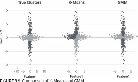
The step-by-step computations performed by the Naïve Bayes (NB) classifier and the Gaussian Mixture Model (GMM) clustering algorithm.
Foundational concepts, such as trial, outcome, and event, along with the differences between the joint and conditional types of probability. For NB—the role of posterior probability, class prior probability, predictor prior probability, and likelihood in solving a classification problem.
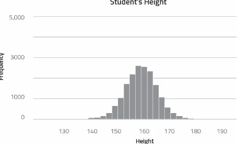
For GMM—the characteristics of a normal distribution and how each distribution can be uniquely identified by its mean and variance parameters. We also consider how GMM uses the two-step expectation maximization optimization technique to assign samples to classes.
We conclude with a hands-on learning section showing how NB and GMM models can be applied to detect spam messages sent via SMS text.
4. Chapter Four: Deep Learning This term encompasses a wide range of learning methods primarily based on the use of neural networks, a class of algorithms so named because they simulate the ways densely interconnected networks of neurons interact in the brain. In this chapter, we consider how two types of neural networks can be applied to solve a classification problem. This includes:
Memory (LSTM) and Convolutional (CNN) types of neural networks.
Foundational concepts, such as nodes, hidden layers, hidden states, activation functions, context, learning rates, dropout regularization, and increasing levels of abstraction.
The differences between feedforward and recurrent neural network architectures and the significance of incorporating fully-connected vs. partially-connected layers.
We conclude with a hands-on learning section showing how LSTM and CNN models can be applied to determine the length of the XOR key used to obfuscate a sample of text.
We strongly believe there’s no substitute for practical experience. Consequently, we’re making all the scripts and datasets we demonstrate in the hands-on learning sections available for download at:
https://www.cylance.com/intro-to-ai
For simplicity, all of these scripts have been hard-coded with settings we know to be useful. However, we suggest you experiment by modifying these scripts—and creating new ones too—so you can fully appreciate how flexible and versatile these methods truly are.
Clustering
Using the
K
-Means and DBSCAN Algorithms
The purpose of cluster analysis
is to segregate data into a set of discrete groups or clusters based on similarities among their key features or attributes. Within a given cluster, data items will be more similar to one another than they are to data items within a different cluster. A variety of statistical, artificial intelligence, and machine learning techniques can be used to create these clusters, with the specific algorithm applied determined by the nature of the data and the goals of the analyst.Although cluster analysis first emerged roughly eighty-five years ago in the social sciences, it has proven to be a robust and broadly applicable method of exploring data and extracting meaningful insights. Retail businesses of all stripes, for example, have famously used cluster analysis to segment their customers into groups with similar buying habits by analyzing terabytes of transaction records stored in vast data warehouses. Retailers can use the resulting customer segmentation models to make personalized upsell and cross-sell offers that have a much higher likelihood of being accepted. Clustering is also used frequently in combination with other analytical techniques in tasks as diverse as pattern recognition, analyzing research data, classifying documents, and—here at Cylance—in detecting and blocking malware before it can execute.
stepping through this same procedure on your own.
Step 1: Data Selection and Sampling
Before we start with any machine learning approach, we need to start with some data. Ideally, we might wish to subject all of our network operations and system data to analysis to ensure our results accurately reflect our network and computing environment. Often, however, this is neither possible nor practical due to the sheer volume of the data and the difficulty in collecting and consolidating data distributed across heterogeneous systems and data sources. Consequently, we typically apply statistical sampling techniques that allow us to create a more manageable subset of the data for our analysis. The sample should reflect the characteristics of the total dataset as closely as possible, or the accuracy of our results may be compromised. For example, if we decided to analyze Internet activity for ten different computers, our sample should include representative log entries from all ten systems.
Step 2: Feature Extraction
In this stage, we decide which data elements within our samples should be extracted and subjected to analysis. In machine learning, we refer to these data elements as “features,” i.e., attributes or properties of the data that can be analyzed to produce useful insights.
In facial recognition analysis, for example, the relevant features would likely include the shape, size and configuration of the eyes, nose, and mouth. In the security domain, the relevant features might include the percentage of ports that are open, closed, or filtered, the application running on each of these ports, and the application version numbers. If we’re investigating the possibility of data exfiltration, we might want to include features for bandwidth utilization and login times.
Step 3: Feature Encoding and Vectorization
Most machine learning algorithms require data to be encoded or represented in some mathematical fashion. One very common way data can be encoded is by mapping each sample and its set of features to a grid of rows and columns. Once structured in this way, each sample is referred to as a “vector.” The entire set of rows and columns is referred to as a “matrix.” The encoding process we use depends on whether the data representing each feature is continuous, categorical, or of some other type.
Data that is continuous can occupy any one of an infinite number of values within a range of values. For example, CPU utilization can range from 0 to 100 percent. Thus, we could represent the average CPU usage for a server over an hour as a set of simple vectors as shown below.
Sample (Hour) CPU Utilization %
2 AM 12
9 AM 76
1 PM 82
6 PM 20
Unlike continuous data, categorical data is typically represented by a small set of permissible values within a much more limited range. Software name and release number are two good examples. Categorical data is inherently useful in defining groups. For example, we can use categorical features such as the operating system and version number to identify a group of systems with similar characteristics.
Host Ubuntu Red Hat EnterpriseLinux SUSE Linux EnterpriseServer
A 1 0 0
B 0 1 0
C 0 0 1
As we can see, Host A is running Ubuntu while Hosts B and C are running Red Hat and SUSE versions of Linux respectively.
Alternately, we can assign a value to each operating system and vectorize our hosts accordingly:
Operating System Assigned Value Host Vector
Ubuntu 1 A 1
Red Hat Enterprise Linux 2 B 2 SUSE Linux Enterprise Server 3 C 3
However, we must be careful to avoid arbitrary mappings that may cause a machine learning operation, such as a clustering algorithm, to mistakenly infer meaning to these values where none actually exists. For example, using the mappings above, an algorithm might learn that Ubuntu is “less than” Red Hat because 1 is less than 2 or reach the opposite conclusion if the values were reversed. In practice, analysts use a somewhat more complicated encoding method that is often referred to as “one-hot encoding.”
distance from a central point to group vectors by similarity. Without normalization, k-means may overweigh the effects of the categorical data and skew the results accordingly.
Let’s consider the following example:
Sample (Server) Requests per Second CPU Utilization %
Alpha 200 67
Bravo 160 69
Charlie 120 60
Delta 240 72
Here, the values of the Requests per Second feature have a range ten times larger than those of the CPU Utilization % feature. If these values were not normalized, the distance calculation would likely be skewed to overemphasize the effects of this range disparity.
In the chart below, for example, we can see that the difference between server Alpha and server Bravo with respect to Requests per Second is 40, while the difference between the servers with respect to CPU Utilization % is only 2. In this case, Requests per Second accounts for 95% of the difference between the servers, a disparity that might strongly skew the subsequent distance calculations.
We’ll address this skewing problem by normalizing both features to the 0-1 range using the formula: x-xmin / xmax – xmin.
Sample (Name) Requests per Second CPU Utilization %
Alpha .66 .58
Bravo .33 .75
Charlie 0 0
After normalizing, the difference in Requests per Second between servers Alpha and Bravo is .33, while the difference in CPU Utilization % has been reduced to 17. Requests per Second now accounts for only 66% of the difference.
Step 4: Computation and Graphing
Once we finish converting features to vectors, we’re ready to import the results into a suitable statistical analysis or data mining application such as IBM SPSS Modeler and SAS Data Mining Solution. Alternately we can utilize one of the hundreds of software libraries available to perform such analysis. In the examples that follow, we’ll be using scikit-learn, a library of free, open source data mining and statistical functions built in the Python programming language.
Clustering with K-Means
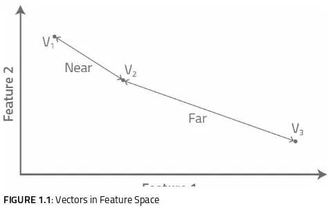
As humans, we experience the world as consisting of three spatial dimensions, which allows us to determine the distance between any two objects by measuring the length of the shortest straight line connecting them. This “Euclidean distance” is what we compute when we utilize the Pythagorean Theorem.
Clustering analysis introduces the concept of a “feature space” that can contain thousands of dimensions, one each for every feature in our sample set. Clustering algorithms assign vectors to particular coordinates in this feature space and then measure the distance between any two vectors to determine whether they are sufficiently similar to be grouped together in the same cluster. As we shall see, clustering algorithms can employ a variety of distance metrics to do so. However, k-means utilizes Euclidean distance alone. In k-means, and most other clustering algorithms, the smaller the Euclidean distance between two vectors, the more likely they are to be assigned to the same cluster.
FIGURE 1.1: Vectors in Feature Space
The version of k-means we’ll be discussing works with continuous data only. (More sophisticated versions work with categorical data as well.) The underlying patterns within the data must allow for clusters to be defined by carving up feature space into regions using straight lines and planes.
The data can be meaningfully grouped into a set of similarly sized clusters.
If these conditions are met, the clustering session proceeds as follows:
1. A dataset is sampled, vectorized, normalized, and then imported into scikit- learn.
2. The data analyst invokes the k-means algorithm and specifies “k,” an input variable or “hyperparameter” that tells k-means how many clusters to create. (Note: Almost every algorithm includes one or more hyperparameters for “tuning” the algorithm’s behavior.) In this example,
k will be set to three so that, at most, three clusters are created.
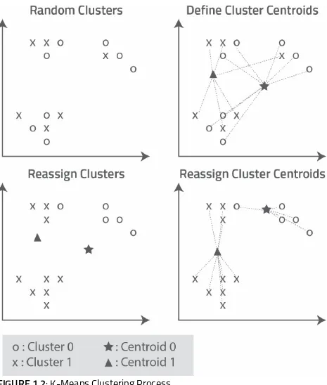
3. K-Means randomly selects three vectors from the data-set and assigns each of them to a coordinate in feature space, one for each of the three clusters to be created. These points are referred to as “centroids.”
4. K-Means begins processing the first vector in the dataset by calculating the Euclidean distance between its coordinates and the coordinates of each of the three centroids. Then, it assigns the sample to the cluster with the nearest centroid. This process continues until all of the vectors have been assigned in this way.
5. K-Means examines the members of each cluster and computes their average distance from their corresponding centroid. If the centroid’s current location matches this computed average, it remains stationary. Otherwise, the centroid is moved to a new coordinate that matches the computed average.
6. K-Means repeats step four for all of the vectors and reassigns them to clusters based on the new centroid locations.
7. K-Means iterates through steps 5-6 until one of the following occurs: The centroid stops moving and its membership remains fixed, a state known as “convergence.”
FIGURE 1.2: K-Means Clustering Process
Once clustering is complete, the data analyst can:
Evaluate the accuracy of the results using a variety of validation techniques.
membership of new samples.
Analyze the cluster results further using additional statistical and machine learning techniques.
This same process applies with higher dimensional feature spaces too—those containing hundreds or even thousands of dimensions. However, the computing time for each iteration will increase in proportion to the number of dimensions to be analyzed.
K
-MEANS PITFALLS AND LIMITATIONS
While it’s easy to use and can produce excellent results, the version of k-means we have been discussing is vulnerable to a variety of errors and distortions:
The analyst must make an informed guess at the outset concerning how many clusters should be created. This takes considerable experience and domain expertise. In practice, it’s often necessary to repeat the clustering operation multiple times until the optimum number of clusters has been identified.
The clustering results may vary dramatically depending on where the centroids are initially placed. The analyst has no control over this since this version of k-means assigns these locations randomly. Again, the analyst may have to run the clustering procedure multiple times and then select the clustering results that are most useful and consistent with the data.
Clustering with DBSCAN
Another commonly used clustering algorithm is DBSCAN or “Density-Based Spatial Clustering of Applications with Noise.” DBSCAN was first introduced in 1996 by Hans-Peter Kriegel.
As the name implies, DBSCAN identifies clusters by evaluating the density of points within a given region of feature space. DBSCAN constructs clusters in regions where vectors are most densely packed and considers points in sparser regions to be noise.
In contrast to k-means, DBSCAN:
Discovers for itself how many clusters to create rather than requiring the analyst to specify this in advance with the hyperparameter k.
Is able to construct clusters of virtually any shape and size.
DBSCAN presents the analyst with two hyperparameters that determine how the clustering process proceeds:
Epsilon (Eps) specifies the radius of the circular region surrounding each point that will be used to evaluate its cluster membership. This circular region is referred to as the point’s “Epsilon Neighborhood.” The radius can be specified using a variety of distance metrics.
Minimum Points (MinPts) specifies the minimum number of points that must appear within an Epsilon neighborhood for the points inside to be included in a cluster.
DBSCAN performs clustering by examining each point in the dataset and then assigning it to one of three categories:
A core point is a point that has more than the specified number of MinPts within its Epsilon neighborhood.
A border point is one that falls within a core point’s neighborhood but has insufficient neighbors of its own to qualify as a core point.
FIGURE 1.3: DBSCAN Clustering Process
A DBSCAN clustering session in scikit-learn typically proceeds as follows: 1. A dataset is sampled, vectorized, normalized, and then imported into
scikit-learn.
2. The analyst builds a DBSCAN object and specifies the initial Eps and MinPts values.
3. DBSCAN randomly selects one of the points in the feature space, e.g., Point A, and then counts the number of points—including Point A—that lie within Point A’s Eps neighborhood. If this number is equal to or greater than MinPts, then the point is classified as a core point and DBSCAN adds Point A and its neighbors to a new cluster. To distinguish it from existing clusters, the new cluster is assigned a cluster ID.
visited all of the neighbors and detected all of that cluster’s core and border points.
5. DBSCAN moves on to a point that it has not visited before and repeats steps 3 and 4 until all of the neighbor and noise points have been categorized. When this process concludes, all of the clusters have been identified and issued cluster IDs.
If the results of this analysis are satisfactory, the clustering session ends. If not, the analyst has a number of options. They can tune the Eps and MinPts hyperparameters and run DBSCAN again until the results meet their expectations. Alternately, they can redefine how the Eps hyperparameter functions in defining Eps neighborhoods by applying a different distance metric. DBSCAN supports several different ones, including:
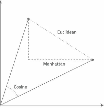
Euclidean Distance This is the “shortest straight-line between points” method we described earlier.
Manhattan or City Block Distance As the name implies, this method is similar to one we might use in measuring the distance between two locations in a large city laid out in a two-dimensional grid of streets and avenues. Here, we are restricted to moving along one dimension at a time, navigating via a series of left and right turns around corners until we reach our destination. For example, if we are walking in Manhattan from Third Avenue and 51st Street to Second Avenue and 59th Street, we must
travel one block east and then eight blocks north to reach our destination, for a total Manhattan distance of nine blocks. In much the same way, DBSCAN can compute the size of the Eps neighborhood and the distance between points by treating feature space as a multi-dimensional grid that can only be traversed one dimension at a time. Here, the distance between points is calculated by summing the number of units along each axis that must be traversed to move from Point A to Point B.
point. The smaller the angle, the more likely the two points are to have similar features and live in the same Eps neighborhood. Likewise, the larger the angle, the more likely they are to have dissimilar features and belong to different clusters.
FIGURE 1.4: Euclidean, Manhattan, and Cosine Distances
DBSCAN PITFALLS AND LIMITATIONS
Is extremely sensitive to even small changes in MinPts and Eps settings, causing it to fracture well-defined clusters into collections of small cluster fragments.
Becomes less computationally efficient as more dimensions are added, resulting in unacceptable performance in extremely high dimensional feature spaces.
Assessing Cluster Validity
At the conclusion of every clustering procedure, we’re presented with a solution consisting of a set of k clusters. But how are we to assess whether these clusters are accurate representations of the underlying data? The problem is compounded when we run a clustering operation multiple times with different algorithms or the same algorithm multiple times with different hyperparameter settings.
Fortunately, there are numerous ways to validate the integrity of our clusters. These are referred to as “indices” or “validation criteria.” For example, we can:
Run our sample set through an external model and see if the resulting cluster assignments match our own.
Test our results with “hold out data,” i.e., vectors from our dataset that we didn’t use for our cluster analysis. If our cluster results are correct, we would expect the new samples to be assigned to the same clusters as our original data.
Use statistical methods. With k-means, for example, we might calculate a Silhouette Coefficient, which compares the average distance between points that lie within a given cluster to the average distance between points assigned to different clusters. The lower the coefficient, the more confident we can be that our clustering results are accurate.
Cluster Analysis Applied to Real-World Threat Scenarios
As we’ve seen, cluster analysis enables us to examine large quantities of network operations and system data in order to detect hidden relationships among cluster members based on the similarities and differences among the features that define them. But, how do we put these analytical capabilities to work in detecting and preventing real-world network attacks? Let’s consider how cluster analysis might have been useful with respect to the Panama Papers breach, which resulted in the exfiltration of some 11.5 million confidential documents and 2.6 terabytes of client data from Panamanian law firm Mossack Fonseca (MF).
We begin with three caveats:
Although compelling evidence has been presented by various media and security organizations concerning the most likely attack vectors, no one can say with certainty how hacker “John Doe” managed to penetrate MF’s web server, email server, and client databases over the course of a year or more. We would have to subject MF’s network and system data to an in-depth course of forensic analysis to confirm the nature and extent of these exploits.
This data would have to be of sufficient scope and quality to support the variety of data-intensive methods we commonly employ in detecting and preventing attacks.
Our analysis would not be limited to clustering alone. Ideally, we would employ a variety of machine learning, artificial intelligence, and statistical methods in combination with clustering.
For now, however, we’ll proceed with a clustering-only scenario based on the evidence presented by credible media and industry sources.
plugin, which MF used for its email list management capabilities. Collectively, these and other mail server hacks would have enabled John Doe to access and exfiltrate huge quantities of MF emails.
Forbes Magazine9 has also reported that, at the time of the attack, MF was
running Drupal version 7.23 to manage the “secure” portal that clients used to access their private documents. This version was widely known to be vulnerable to a variety of attacks, including an SQL injection exploit that alone would have been sufficient to open the floodgates for a mass document exfiltration.
Based on this and other information, we find it likely that cluster analysis— pursued as part of an ongoing hunting program—could have detected anomalies in MF’s network activity and provided important clues about the nature and extent of John Doe’s attacks. Normally, hunt team members would analyze the web and mail server logs separately. Then, if an attack on one of the servers was detected, the hunt team could analyze data from the other server to see if the same bad actors might be involved in both sets of attacks and what this might indicate about the extent of the damage.
On the mail server side, the relevant features to be extracted might include user login time and date, IP address, geographic location, email client, administrative privileges, and SMTP server activity. On the web server side, the relevant features might include user IP address and location, browser version, the path of the pages being accessed, the web server status codes, and the associated bandwidth utilization.
After completing this cluster analysis, we would expect to see the vast majority of the resulting email and web vectors grouped into a set of well-defined clusters that reflect normal operational patterns and a smaller number of very sparse clusters or noise points that indicate anomalous user and network activity. We could then probe these anomalies further by grepping through our log data to match this suspect activity to possible bad actors via their IP addresses.
This analysis could reveal:
Anomalous user behavior. We might identify clusters of clients who log in and then spend long hours downloading large quantities of documents without uploading any. Alternately, we might find clusters of email users spending long hours reading emails but never sending any.
Anomalous network traffic patterns. We might observe a sharp spike in the volume of traffic targeting the client portal page and other URLs that include Drupal in their path statements.
Clustering Session Utilizing HTTP Log Data
Let’s apply what we’ve learned to see how clustering can be used in a real-world scenario to reveal an attack and track its progress. In this case, we’ll be analyzing HTTP server log data from secrepo.com that will reveal several exploits similar to those that preceded the Panama Papers exfiltration. If you’d
like to try this exercise out for yourself, please visit
https://www.cylance.com/intro-to-ai, where you’ll be able to download all of the pertinent instructions and data files.
HTTP server logs capture a variety of useful forensic data about end-users and their Internet access patterns. This includes IP addresses, time/date stamps, what was requested, how the server responded, and so forth. In this example, we’ll cluster IP addresses based on the HTTP verbs (e.g., GET, POST, etc.) and HTTP response codes (e.g., 200, 404, etc.). We’ll be hunting for evidence of a potential breach after receiving information from a WAF or threat intelligence feed that the IP address 70.32.104.50 has been associated with attacks targeting WordPress servers. We might be especially concerned if a serious WordPress vulnerability, such as the Revolution Slider, had recently been reported. Therefore, we’ll cluster IP addresses to detect behavior patterns similar to those reported for 70.32.104.50 that might indicate our own servers have been compromised.
The HTTP response codes used for this specific dataset are as follows:
200, 404, 304, 301, 206, 418, 416, 403, 405, 503, 500
The HTTP verbs for this specific dataset are as follows:
GET, POST, HEAD, OPTIONS, PUT, TRACE
We’ll run our clustering procedure twice, once with k-means and then a second time with DBSCAN. We’ll conclude each procedure by returning to our log files and closely examining the behavior of IP addresses that appear as outliers or members of a suspect cluster.
CLUSTER ANALYSIS WITH
K
-MEANS
We begin by preparing our log samples for analysis. We’ll take a bit of a shortcut here and apply a script written expressly to vectorize and normalize this particular dataset.
For each IP address, we’ll count the number of HTTP response codes and verbs. Rather than simply adding up the number of occurrences, however, we’ll represent these features as continuous values by normalizing them. If we didn’t do this, two IPs with nearly identical behavior patterns might be clustered differently simply because one made more requests than the other.
Given enough time and CPU power, we could examine all 16,407 IP addresses in our log file of more than 181,332 entries. However, we’ll begin with the first 10,000 IP addresses instead and see if this sample is sufficient for us to determine whether an attack has taken place. We’ll also limit our sample to IP addresses associated with at least five log entries each. Those with sparser activity are unlikely to present a serious threat to our web and WordPress servers.
The following Python script will invoke the vectorization process:
`python vectorize_secrepo.py`
This produces “secrepo.h5,” a Hierarchical Data Format (HDF5) file that contains our vectors along with a set of cluster IDs and “notes” that indicate which IP address is associated with each vector. We’ll use these addresses later when we return to our logs to investigate potentially malicious activity.
Step 2: Graphing Our Vectors
We’re ready now to visualize our vectors in feature space.
more convenient to prepare several viewing angles in advance during the graphing process. Subsequently, we can toggle quickly between each of the prepared views to view our clusters from different angles.
We’ll use the following script to visualize our vectors:
`python visualize_vectors.py -i secrepo.h5`
FIGURE 1.6: Projected Visualization of Our Vectors
Step 3: First Pass Clustering with K-Means
As noted earlier, k-means only requires us to set the hyperparameter k, which specifies how many clusters to create. We won’t know initially what the correct value of k should be. Therefore, we’ll proceed through the clustering process iteratively, setting different k values and inspecting the results until we’re satisfied we’ve accurately modeled the data. We’ll begin by setting k to “2.” We’ll also instruct k-means to use the cluster IDs we specified during vectorization to name each cluster:
`python cluster_vectors.py -c kmeans -n 2 -i secrepo.h5 -o secrepo.h5`
Step 4: Validating Our Clusters Statistically
Now that we have the cluster IDs, we can determine how well our samples have been grouped by applying Silhouette Scoring. The scores will range from -1 to +1. The closer the scores are to +1, the more confident we can be that our grouping is accurate.
We’ll produce the Silhouette Scores with the following script:
stats_vectors.py
As we can see, Cluster 1 is well-grouped while Cluster 0 is not. We also notice that Cluster 1 contains many more samples than Cluster 0. We can interpret this to mean that Cluster 1 reflects normal network activity while Cluster 0 contains less typical and possibly malicious user behavior.
Step 5: Inspecting Our Clusters
We can now interrogate our clusters to see which one contains the IP address of our known bad actor. We’ll use the following script to print out the labels and notes for each of our vectors.
We can now see that IP 70.32.104.50 is a member of Cluster 0—our suspect cluster—and the one with the lower average silhouette score. Given this result, we might consider subjecting all of Cluster 0’s members to forensic analysis. However, human capital is expensive and investigating all of these IPs would be inefficient. Therefore, it makes better sense for us to focus on improving our clustering results first so we have fewer samples to investigate.
Step 6: Modifying K to Optimize Cluster Results
Generally speaking, it makes sense to start a k-means clustering session with k
set to construct at least two clusters. After that, you can iterate higher values of k
until your clusters are well formed and validated to accurately reflect the distribution of samples. In this case, we performed steps three and four multiple times until we finally determined that 12 was the optimal number for this dataset.
We’ll go ahead and generate these 12 clusters with the following script:
`python cluster_vectors.py -c kmeans -n 12 -i secrepo.h5 -o secrepo.h5`
Step 7: Repeating Our Inspection and Validation Procedures
Once again, we’ll run a script to extract the ID for the cluster that now contains the malicious IP:
`python label_notes.py -i secrepo.h5 | grep 70.32.104.50`
`python stats_vectors.py secrepo.h5`
As we can see, Cluster 6 has a high Silhouette Score, indicating that all of the members are highly similar to one another and to the IP we knew at the outset to be malicious. Our next step should be to see what these IP addresses have been doing by tracking their activity in our web server logs. We’ll begin by printing out all of the samples in Cluster 6 using the following command:
Now, we can use the grep command to search through our logs and display entries in which these IP addresses appear. We’ll start with our known bad IP:
As we can see, this IP has been attempting to exploit remote file inclusion vulnerabilities to install a PHP script payload. Now let’s try another member of the suspect cluster:
`grep -ar 49.50.76.8 datasets/http/secrepo/www.secrepo.com/self.logs/`
CLUSTER ANALYSIS WITH DBSCAN
Since we’ve already created the secrepo.h5 file for our k-means example, we’ll skip ahead to Step 3 and begin our first-pass clustering session with DBSCAN. We’ll start by setting the Eps and MinPts hyperparameters to 0.5 and 5 respectively. As noted earlier, DBSCAN doesn’t require us to predict the correct number of clusters in advance. It will compute the quantity of clusters on its own based on the density of vectors in feature space and the minimum cluster size.
To generate these clusters we’ll run the following script:
`python cluster_vectors.py -c dbscan -e 0.5 -m 2 -i secrepo.h5 -o secrepo.h5`
unassigned. Each of these 854 noise points may be associated with malicious activity. We could return to our logs now and investigate all of them but this would be time consuming and inefficient. Instead, we’ll increase our Eps setting from 5 to 6. This should produce fewer clusters and also a smaller quantity of potentially suspect samples.
We’ll apply the new hyperparameter settings with the following command:
`python cluster_vectors.py -c dbscan -e 6 -m 5 -i secrepo.h5 -o secrepo.h5`
This time, DBSCAN generated 11 clusters and only 25 noise points, a much more manageable number. We’ll skip the cluster inspection and validation steps we described previously for k-means and jump ahead to begin investigating the behavior of these 25 suspect samples. We’ll start by listing these samples with the following command:
Now, we can use the following script to grep through our log files and find out what these IPs have been doing:
`grep -ar 192.187.126.162 datasets/http/secrepo/www.secrepo. com/self.logs/`
Clustering Takeaways
As we’ve seen, clustering provides a mathematically rigorous approach to detecting patterns and relationships among network, application, file, and user data that might be difficult or impossible to secure in any other way. However, our analytical story only begins with clustering. In the chapters to come, we’ll describe some of the other statistical, artificial intelligence, and machine learning techniques we commonly employ in developing and deploying our network security solutions. For now, however, here are your key clustering takeaways:
Cluster analysis can be applied to virtually every kind of data once the relevant features have been extracted and normalized.
In cluster analysis, similarity between samples and their resulting cluster membership is determined by measuring the distance between vectors based on their locations in feature space. A variety of distance metrics can be applied, including Euclidean, Manhattan, Cosine, and more.
K-means and DBSCAN are easy to use, computationally efficient and broadly applicable to a variety of clustering scenarios. However, both methods are vulnerable to the “curse of dimensionality” and may not be suitable when analyzing extremely high dimensional feature spaces.
Clustering results must be statistically validated and also carefully evaluated with respect to real-world security threats. This requires a significant amount of domain expertise and a deep understanding of the capabilities, pros, and cons of each clustering method.
Classification
Using the Logistic Regression and Decision Tree Algorithms
We humans employ a wide
variety of cognitive strategies to make sense of the world around us. One of the most useful is our capacity to assign objects and ideas to discrete categories based on abstract relationships among their features and characteristics. In many cases, the categories we use are binary ones. Certain foods are good to eat, others are not. Certain actions are morally right while others are morally wrong. Categories like these enable us to make generalizations about objects and actions we already know about in order to predict the properties of objects and actions that are entirely new to us.Presented with an oval object with a yellow skin, a soft interior, and a sweet and pungent smell, we might draw on our past knowledge to predict that it belongs to the category “fruit.” We could test the accuracy of our prediction by bringing the object to a fruit store. If we found a bin full of similar objects labeled as “mangos” we could conclude that our prediction was a correct one. If so, we could generalize from our knowledge of fruit to predict that the mango has a pleasant taste and offers sound nutritional benefits. We could then apply this categorical knowledge to decide whether to eat the mango. This process of assigning an unknown object to a known category in order to make informed decisions is what we mean by the term classification.
connection is benign or associated with a botnet. These are examples of a binary classification problem—for example, one with only two output classes, “spam” and “not spam,” “botnet” or “benign.” By convention, samples that possess the attribute we’re investigating (e.g., that an email is spam) are labeled as belonging to class “1” while samples that don’t possess this attribute (e.g., mail that is not spam) are labeled as belonging to class “0.” These 1 and 0 class labels are often referred to as positive and negative cases respectively.
Classification can also be used with problems in which:
A sample can belong to multiple classes at the same time. For example, the mango we identified earlier could be assigned labels corresponding to the classes of fruit, yellow, tropical, etc.
We are performing multinomial—rather than binary—classification. In this case, a sample is assigned to one class among a set of three or more. For example, we might want to classify an email sample as either belonging to class 1 (benign), class 2 (spam), or class 3 (a phishing exploit).
For the purposes of this chapter, however, we’ll consider binary classification problems only.
Supervised Vs. Unsupervised Learning
Classification is an example of supervised learning, in which an analyst builds a model with samples that have already been identified—or labeled—with respect to the property under investigation. In the case of spam, for example, the analyst builds a classification model using a dataset of samples that have already been labeled as either spam (the positive case) or not spam (the negative case). Here, the job of the classifier is to ascertain how the feature attributes of each class can be used to predict the class of new, unlabeled samples. In contrast, clustering is an example of unsupervised learning, in which the properties that distinguish one group of samples from another must be discovered.
It’s not uncommon to use unsupervised and supervised methods in combination. For example, clustering can be used to segregate network traffic vectors into distinct groups. Then, members of the forensic team can investigate members of suspect clusters to see if they have performed some kind of undesirable network activity. If so, the vectors associated with this activity can be labeled as belonging to class 1 (e.g., as botnet traffic) while all of the other vectors can be labeled as class 0 (e.g., as benign activity). Once labeled, the vectors can be used by a classifier to construct a model that predicts whether a new unlabeled vector is benign or a member of a bot network.
To produce an accurate model, analysts need to secure a sufficient quantity of data that has been correctly sampled, vectorized, and labeled. This data is then typically divided into two or three distinct sets for training, validation, and testing. Splitting into three sets is preferable when there is sufficient data available. In either case, the training set is typically the largest subset, comprising between 70-90% of the total samples. As a rule of thumb, the larger the training set, the more likely the classifier is to produce an accurate model. However, enough testing data must always be retained to conduct a reliable assessment of the model’s accuracy.
A classification session typically proceeds through four phases:
control how the resulting models are built.
2. A validation phase in which the analyst applies the validation data to the model in order to assess its accuracy and utilizes various procedures for optimizing the algorithm’s hyperparameter settings. To learn about these optimization methods, please refer to the links provided in the resources section at the end of this chapter.
3. A testing phase to assess the model’s accuracy with test data that was withheld from the training and validation processes. The analyst runs the test vectors through the model and then compares each test sample’s predicted class membership to its actual class membership. If the results meet the required accuracy and performance thresholds, the analyst can proceed to the deployment phase. Otherwise, they can return to the training phase to refine and rebuild the model.
4. A deployment phase, in which the model is applied to predict the class membership of new, unlabeled data.
In practice, an analyst may train and test multiple models using different algorithms and hyperparameter settings. Then, they can compare the models and choose the one that offers the optimal combination of accuracy as well as the most efficient use of computing resources.
Classification Challenges
Classifiers can often produce excellent results under favorable conditions. However, this is not always the case. For example:
It can be extremely difficult for analysts to obtain a sufficiently large and accurately classified set of labeled data.
Classification via Logistic Regression (LR)
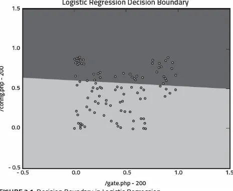
In the previous chapter, we introduced the concept of feature space and described how groups of vectors can be assessed for similarity based on the distance between them and their nearest neighbors. Feature space plays a role in logistic regression too, however the mechanisms used to assess similarity and assign vectors to classes operate somewhat differently.
FIGURE 2.1: Decision Boundary in Logistic Regression
LR includes several different solver functions for determining the location of the decision boundary and assigning vectors to classes. In the discussion below, we’ll describe the liblinear solver and how it applies the coordinate descent
method to accomplish this.
THE ROLE OF REGRESSION WEIGHTS
Regression weights play a central role in determining how much each feature and feature value contributes to a given vector’s class membership. This is achieved by multiplying each feature value by its corresponding weight as shown below.
Feature 1 Feature 2 Feature 3
Regression Weight 0.05 75 -6 Product 12.5 1050 -252
Positive and negative weight values contribute to class 1 and class 0 classifications respectively. As we can see, the large positive value of Feature 1 could indicate that it has a strong influence on the prediction that this sample belongs to the positive class. However, Feature 1’s impact is significantly diminished by its low regression weight. Consequently, Feature 1 can now be seen to make only a small contribution to this sample’s potential to be labeled as class 1. In contrast, the contribution of Feature 2 has been significantly increased due to its much larger regression weight. In turn, Feature 3’s influence has been increased six-fold, but in the direction of predicting a negative class membership.
In practice, the product of a single feature value/regression weight combination is likely to have only a negligible effect in predicting a sample’s class membership since each vector may contain values for hundreds or even thousands of features. Instead, it is the aggregate of these calculations that is significant.
To predict a class, LR sums all of the products together with a computed bias
value. If the aggregate sum is greater than or equal to zero, LR will predict the sample as belonging to class 1. If the sum is less than zero, LR will predict the sample as a class 0 member. In our hypothetical example, LR adds our bias value (+5) to the sum of our vector products (12.5) + (1050) + (-252) for a total of 815.5. Since the sum is greater than zero, our sample would be predicted as belonging to Class 1. We could now compare the sample’s predicted class membership to its actual class membership to see if our regression weights were correct.
Most of the training phase of an LR session is devoted to optimizing these weights. First, however, an initial set of weights must be applied. There are numerous methods for doing so. For example, starting weight values can be set arbitrarily using a random number generator. Ultimately, the classifier will almost always compute the optimal values given enough computing time.
THE ROLE OF REGULARIZATION AND PENALTY PARAMETERS
modeling results, a problem analysts commonly address through normalization. Similar distortions can be caused by regression weights with very large values. Consequently, the LR algorithm provides a number of penalty parameters that analysts can use to mitigate these effects.
For example, analysts can use the penalty parameter C to compress the range of regression weights in much the same way they use normalization to compress feature values. This process is referred to as regularization. C controls how large the weight values can become. Models with extremely high weight ranges may do an excellent job in predicting the class of training vectors but produce subpar results when applied to test data. Models like these are said to over-fit the data. This disparity in a model’s accuracy can be an important clue to the analyst that more aggressive regularization is needed.
Regularization can also be useful when the analyst suspects that a solver is focusing excessively on a small set of highly influential features. By regularizing, the analyst can force the solver to incorporate additional features in a controlled and measured way.
Regularization can also be used to control which features are allowed to influence the classifier in computing regression weights. This is accomplished utilizing the penalty parameters L1 and L2. The two parameters operate somewhat differently. L1 sets a threshold that determines how aggressive LR should be in eliminating features with comparatively low predictive power. The higher the weight assigned to L1, the more features will be excluded. In contrast, L2 minimizes the impact of a group of highly correlated features so that their collective influence does not skew the results.
Let’s take a look now at the sequence of steps and methodology that comprise the training phase of a typical logistic regression session with scikit-learn.
LOGISTIC REGRESSION TRAINING PHASE
During this phase, the analyst’s primary goal is to fit the data by producing an optimized set of regression weights. During the subsequent testing phase, the weights will be applied to predict each test vector’s class membership. Next, the results will be subjected to validation functions that determine how accurately the predicted class assignments match the known class labels.
The analyst begins by importing two files:
1. A matrix of normalized training samples.
2. A vector of labels that define each sample’s class membership.
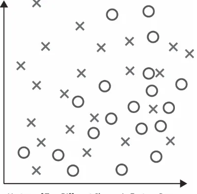
As shown below, each vector can be represented graphically as a point in feature space such that its class membership is indicated visually.
FIGURE 2.2: Labeled Vectors in Feature Space
Step 2: Regularization and Regression Weight Optimization
An initial set of regression weights are assigned, and the analyst invokes a
score is used to calculate a positive or negative adjustment to each weight’s value. The analyst can control the size of this adjustment on a feature-by-feature basis by utilizing a learning rate parameter.
Over the course of repeated calculation cycles, the regression weights will gradually and incrementally move closer and closer to their optimal values. After each optimization, the analyst can experiment with different penalty parameter settings and then assess the resulting model.
However, this brute force approach to optimization is both computation- and time-intensive. At some point, the incremental improvements in model accuracy may no longer justify additional refinements. When that occurs, the analyst may elect to end the training process and move on to the testing phase.
Step 3: Assigning Probability Scores to Class Predictions
Recall that a vector’s classification is computed by summing all of its feature value/weight products together with the bias value and that the vector is assigned to class 1 if the sum is equal to or greater than zero and to class 0 if it is not. However, LR is intrinsically a method for predicting the probability that a given vector belongs to a particular class. Therefore, LR includes a logit function that converts the classification result into a point along a probability curve that ranges from zero to one as shown below.
The closer the point is to a probability score approaching y=1, the stronger the prediction will be that the sample belongs to class 1 (the positive case). Likewise, the closer the point is to p=0, the more strongly it will be predicted to belong to class 0 (the negative case). Results that approach the p=.5 points from either direction become increasingly ambiguous with respect to class predictions. As shown above, the decision boundary is represented by the p=.5 location along the probability curve. If a sample were to land on this coordinate, then it would be equally likely to belong to either class, making a confident prediction impossible.
Step 4: Exporting the Logistic Regression Model
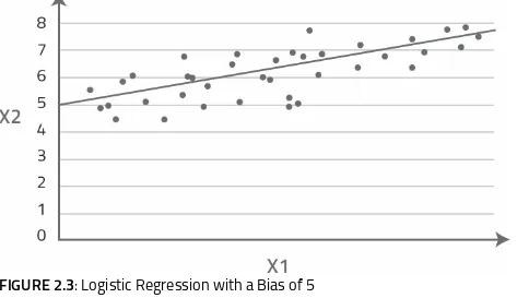
+b in which x1 and x2 are the feature values, m1 and m2 are their respective regression weights and b is the bias value.
In practice, however, this equation is expanded to sum the products of every regression weight/feature value combination. The shape of the resulting decision boundary is determined by the number of features being used for classification. If there are two features, the decision boundary will comprise a line. If there are three dimensions, it will comprise a plane. In higher dimensional spaces than these, the decision boundary will comprise a hyperplane, with one dimension added for each additional feature.
If a non-zero bias value has been computed, the origin point for this decision boundary will be shifted by the number of units specified. In the example below, the origin point for the decision boundary has been shifted five units up along the x2 axis.
FIGURE 2.3: Logistic Regression with a Bias of 5