Volume 10 Number 2 2011
Master of Science in Management, School of Business and Management Institut Teknologi Bandung
Abstract
This paper proposes a government bond portfolio stochastic simulation using a Vasicek Model, a generally used model of term structure of interest rates. The model is used to generate the possible term structure of interest rates for five years based on the historical term structure. The future government debts are forecasted using ARIMA model, and the efficient frontier of costs resulting from portfolios of bond with different maturity structures are determined from the Cost-at-Risk framework. An optimization process will be conducted on the government bond portfolio efficient frontier based on the government risk preference.
Keywords: Yield Curve, Vasicek Model, ARIMA, Cost-at-Risk, financing strategy, maturity
1. Introduction
Bond portfolio optimization is compulsory for a government to attain the lowest possible cost at a permissible interest rate risk level for financing its excess of expenditure. Portfolio management problem can be seen as a multi-period dynamic decision where transactions take place at discrete points in time. At each point, the decision maker has to assess the market condition i.e., interest rates, price, etc and the composition of portfolio (Zenios et al, 1998). Simulation of a debt strategy will help the government manage the financing of its borrowing requirement at the lowest possible cost and risks (Bolder, 2002).
Unlike what have been done by Zenios (1998), Bolder (2002), Danish National Bank (1999), and Hahm and Kim (2003) the financing requirements of Indonesian government being analyzed from 2011 through 2015.
This multiyear analysis mainly based on Indonesia political regime cycle. The Vasicek model is utilized to simulate the movement of short-rate and the evolution of term structure of interest rates as well. A stochastic simulation is constructed based on the financing requirement and the evolution of the term structure of interest rates to find the costs associated with the bond portfolio and the nature of risk associated to it. The costs incurred with the yield curve volatility of respective financing strategies taken by the government re analyzed from Cost-at-Risk framework.
The objective of this paper is to find the frontier of the bond portfolio costs with respect to different maturity structures and interest rate levels. Previous researches by the Danish National Bank (1999), and Hahm and Kim (2003) incorporate only one year horizon in their analysis. In this research, the government financing requirements for five years are forecasted using ARIMA model and the stochastic simulation will consider 5-year investment horizon, and the 5-year financing strategies that constitute the efficient frontier of the Relative Cost-at-Risk are selected as the possible optimum financing strategies.
2. Government Financing Requirement
As the primary input for the yield curve model, the government financing requirements are forecasted for five consecutive years using Autoregressive Moving Average (ARIMA) model (Box-Jenkins method) and then the debt-to-GDP ratio resulting from the forecasts will be compared to the Indonesian government official projection to assess the plausibility of the financing requirement forecast. The financing requirement forecast is very crucial in determining the financing strategy the government will take in issuing their bonds and also the amount of debt service charges incurred in the bonds issuance.
A. ARIMA Forecast
Data for ARIMA Forecast consist of the amount of the government bond from 1998 through 2010 and the Indonesian GDP within the same period in order to assess the plausibility of the forecast result with the Indonesian government's bond projection.
Table 1. Data for ARIMA Forecast
Year Total
The stationarity of the government bond time series is evaluated by performing a unit root test ( Dickey-Fuller Test) to find whether the series contains a unit root or not. When the series are non-stationary data, then differencing process (subtracting xt with xt-1) is conducted until the differenced series contains no unit roots (stationary) and ready for the identification of p and q in the model with the AIC.
Table 2. Unit Root Test on the Government Bond Time Series
t-S tat istic Prob. Augmented Dickey-F uller test statistic -0.471036 0.8546 Test critica l va lues: 1% leve l -4.420595
5% leve l -3.259808 10% le vel -2.771129
Table II shows the null hypothesis that the government bond time series has a unit root is accepted at all critical values. Hence, the time series will be differenced once and the unit root test will be performed, these steps will be conducted for d times until the d-times differenced series contains no unit root and hence exhibits stationary.
Table 3. Unit Root Test on the Government Bond Time Series' First Difference
t-Statistic Prob.
Augmented Dickey-Fuller test statistic -2.069650 0.2578
Test critical values: 1% level -4.420595
5% level -3.259808
10% level -2.771129
Even at the first difference, the null hypothesis that the government bond time series has a unit root is still accepted at all critical values. Thus, a second differencing must be conducted.
Table 4. Unit Root Test on the Government Bond Time Series' Second Difference
t-Statistic
Prob.*
Augmented Dickey-Fuller test statistic -4.886592 0.0044
Test critical values: 1% level -4.297073
5% level -3.212696
10% level -2.747676
The unit root test on the second difference shows that the series has no unit roots and thus is stationary. So, the ARIMA model is ARIMA (p, 2, q) and the values of p and q can be determined by examining the autocorrelations and partial correlations of the second difference and from its AIC.
Figure 1. Autocorrelations and Partial Correlations of the Indonesian government bond time series' second difference
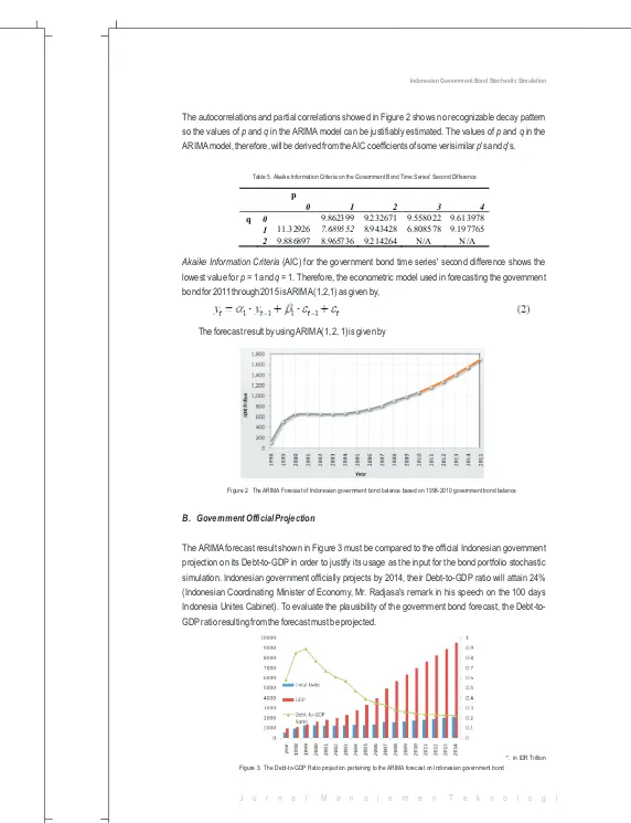
The autocorrelations and partial correlations showed in Figure 2 shows no recognizable decay pattern so the values of p and q in the ARIMA model can be justifiably estimated. The values of p and q in the ARIMA model, therefore, will be derived from the AIC coefficients of some verisimilar p's and q's.
Table 5. Akaike Information Criteria on the Government Bond Time Series' Second Difference
Akaike Information Criteria (AIC) for the government bond time series' second difference shows the lowest value for p = 1 and q = 1. Therefore, the econometric model used in forecasting the government bond for 2011 through 2015 is ARIMA (1,2,1) as given by,
The forecast result by using ARIMA(1, 2, 1) is given by
p
0 1 2 3 4
q 0 9.862399 9.232671 9.558022 9.613978
1 11.32926 7.689552 8.943428 6.808578 9.197765
2 9.886897 8.965736 9.214264 N/A N/A
Figure 2. The ARIMA Forecast of Indonesian government bond balance based on 1998-2010 government bond balance
B. Government Official Projection
The ARIMA forecast result shown in Figure 3 must be compared to the official Indonesian government projection on its Debt-to-GDP in order to justify its usage as the input for the bond portfolio stochastic simulation. Indonesian government officially projects by 2014, their Debt-to-GDP ratio will attain 24% (Indonesian Coordinating Minister of Economy, Mr. Radjasa's remark in his speech on the 100 days Indonesia Unites Cabinet). To evaluate the plausibility of the government bond forecast, the Debt-to-GDP ratio resulting from the forecast must be projected.
Figure 3 shows that the Debt-to-GDP ratio projection in 2014 based on the ARIMA forecast is roughly the same as the Indonesian government planned to be. Therefore the government bond balance forecast in Figure 3 can be justifiably used as the primary input for the government bond portfolio stochastic simulation.
3. Indonesian Government Bond Yield Curve Model
Yield curve is the curve representing the relationship between the maturity of coupon-bearing bonds and their respective yield to maturity (Grandville, 2001) – bonds with different maturities give different levels of yield. A yield curve depicts the yield to maturity of bonds with various maturities. The yield to maturity of a bond is the discount rate which, when applied to each of the bond's cash flows, would make their total present value equal to the cost of the bond (Grandville, 2001). The concept of yield to maturity is, in its essence, analogous to that of Internal Rate of Return (IRR).
In this paper, the yield curve for the Indonesian government bond is modeled using Vasicek Model (Vasicek, 1977), one of the arbitrage approaches to bond pricing together with Cox, Ingersoll, Ross and Brennan, Schwartz. The initial formulation of Vasicek's model is very general, with the short-term interest rate being described by a diffusion process. An arbitrage argument, similar to that used to derive the Black-Scholes option pricing formula (Svoboda, 2003), is applied within this broad framework to determine the partial differential equation satisfied by any contingent claim.
Vasicek model is chosen because of its simplicity and since one of its drawbacks, negative yield to maturity (Hull, 1999), doesn't occur in the modeling of Indonesian government bond – estimations on the model with Indonesian data give an already high short rate, r0 and standard deviation, ó which make it very unlikely for the short rate evolution to reach the value of zero nor even the negative sign.
In the one-factor Vasicek model (Hull, 1999) the risk-neutral process for the short raterr isgiven by
Short rate is a hypothetical interest rate with maturity and a central property to determine the interest rates with real maturities that constitute the yield curve. The yield curve can be thus derived from
where terms A and B are given by
T 0
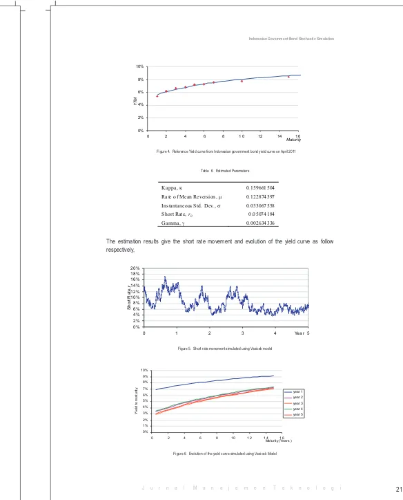
The parameters of the yield curve are estimated using the reference yield curve data on April 2011.
Figure 4. Reference Yield curve from Indonesian government bond yield curve on April 2011 0%
Instantaneous S td. Dev., s 0.033067558
Short Rate, r0 0.05074184
Figure 5. Short rate movement simulated using Vasicek model
0 %
The Vasicek model doesn't only give a plausible forecast of the evolution of yield curve but also provide a range of possible yield curve evolution possibilities. Thousands of possible yield curve evolutions can be generated, each represents a forecast of the yield curve movement. This allows a simulation of how wide the debt service charges of the government bond may vary.
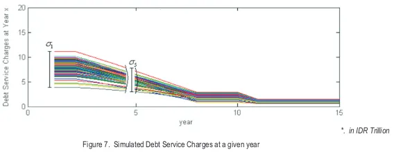
The information of how wide the debt service charge variation gives a reasonable prediction of how much the maximum cost incurred by a financing strategy chosen by the government. Figure 8 shows that as the maturity of a bond lengthens, the lower variation of the interest rates simulated at one maturity date. Short maturity bonds yield lower interest rates but on the other hand more volatile while longer maturity bonds yield more stable interest rates but compensated by higher interest rates.
*. in IDR Trillion
Figure 7. Simulated Debt Service Charges at a given year
The Debt Service Charge here is the amount of yield to maturity times the bond principal that the government must pay each year (in currency unit) as the consequence of the issuance of their bonds. The yield to maturity is a more justifiable approach for financial decision rather than the coupon paid (Brealey, 2003). Hence, the amount of the Debt Service Charge in this paper is calculated from the yield to maturity rather than the amount of coupon payment.
4. Indonesian Government Bond Cost-at-Risk
Cost-at-Risk is a supplementary measure used in the management of the interest-rate risk on the domestic central-government debt (Bolder, 1999). Cost-at-Risk quantifies the risk on the debt and gives important input to the weighing of interest-rate risk against costs. CaR is used in risk management to e.g. assess the consequences of various issuing strategies for the risk on the debt.
The marked part of the right-hand "tail" in the distribution indicates the level of the costs in the (significance level) of cases where costs are highest, the probability where the costs will not exceed the Absolute Cost-at-Risk for the debt. Relative Cost-at-Risk measures the difference between Absolute Cost-at-Risk and the average costs. Relative Cost-at-Risk thereby indicates the maximum deviation from the expected cost at a given confidence level (1 - = 95%, or 1 - = 99%).
Figure 8. Relative Cost-at-Risk indicates the maximum deviation from the expected cost at a given confidence level
Before the simulation results of the Debt Service Charges can be analyzed from the Cost-at-Risk framework, it is mandatory to perform normality test on the results – to see whether the distribution of the data exhibits normality or not. There are at least three tests that must be conducted on the data to ensure the normality of their distributions i.e., symmetry test, whether the mean equals the median, then the Jarque-Bera test that assesses the normality of the distribution from the distribution's kurtosis and skewness, and finally the Kolmogorov-Smirnov test that assesses the cumulative distribution.
In this paper, at least 2,000 simulations are performed for each financing strategy set. If necessary, the number of simulations is increased to met the normality criteria. There are 10 portfolio options for one
5
year and 10 financing strategy combinations for 5 years.
Figure 9 indicates that bonds with shorter maturity on one hand gives lower expected cost, but the other hand gives higher Relative Cost-at-Risk. Suppose that the government chooses to issue their bonds with 80% short-term bonds, the expected cost they have to pay at year 1 will be IDR 5.25 Trillion but they're exposed to IDR 2.8 Trillion Cost-at-Risk. On the contrary if the government chooses to issue 100% bonds on long-term and medium-term, the expected cost will be as high as IDR 6.25 Trillion. But, at 99% confidence level the maximum amount that the cost may sway will IDR 1.7 Trillion. That is at 99% confidence level they have to pay at maxima IDR 7.95 Trillion.
*. In IDR Trillion Figure 9. Relative Cost-at-Risk of Indonesian Government Bonds with various maturity structures at the first year (at 99% confidence level)
This result concurs the findings of Relative Cost-at-Risk simulation of Danish government bonds by Danish National Bank (1999) and the Korean (RoK) external debt by Hahm and Kim (2003), that the relationship between Relative Cost-at-Risk and the expected cost is almost perfectly linear with a down slope. The reason behind this relationship is because the volatility structure of Vasicek model is sloping down towards its maturity (Puhle, 2007),
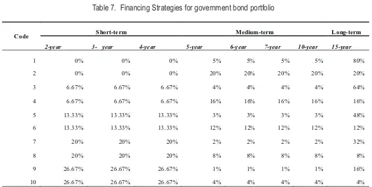
In code '2', still the nothing is allocated for the short-term bond while the 80% of the 100% of portfolio is allocated on medium-term while 20% of the 100% of portfolio is allocated on long-term. The portion for short-term bond increases by 20% incremental for the next 2-pair codes while the rest of portfolio are distributed on the term and long-term with a proportion of 20% of the rest portfolio in medium-term bonds and 80% in long-medium-term bonds for odd codes while 80% of the rest in short-medium-term bonds and 20% in long-term bonds for even codes.
This technique for coding is designed to distinguish the effects of weighting on short-term bonds and those of medium-term as well as long-term bonds. If nothing is allocated on the short-term, is it beneficial from Cost-at-Risk perspective? On the contrary, if most of the portfolio is allocated on the long-term, what are the ramifications on the Cost-at-Risk? Which one is more beneficial for the government, to allocate more on the short-term bonds or on the long-term bonds? Because the analysis is conducted in a 5-year basis, 1 of those 10 portfolios are selected each year and not necessarily the same for every
5
year, e.g. 6-2-7-1-9, or 10-3-8-2-5, or 7-7-7-7-7 – there are 10 possible financing strategy combinations. Each of the portfolio decision yields certain levels of costs until its maturity.
Table 7. Financing Strategies for government bond portfolio
Code S hort-te rm Medium-term L ong- term
The yield to maturity as the basis of the analysis is, in essence, the same as the internal rate of return. To compare investments of different horizon incremental analysis is usually performed to compare investment options. The difference of costs used to analyze the bonds' Cost-at-Risk (Bolder, 2002). The cost of debt is the NPV of the increments of costs incurred by the issuance of each debt during the 5-year administration with Indonesian Central Bank rate (the risk-free rate) is taken as the discount factor,
Relative Cost-at-Risk of the bond is measured from the simulated Cost of Debt.
Figure 10. Efficient frontier of Indonesian government bond cost of debt
Each point in Figure 10 represents the expected value of the 2000+ simulated costs (x-axis) with respect to its Relative Cost-at-Risk (y-axis). The efficient frontier of Indonesian government bond cost of debt is represented by the red line. If the government chooses a financing strategy outside the red line it will give too high cost for the level of risk.
Table 8. Efficient Frontier of Government Bond Portfolio
Financing Strategy expec te d
c os t
Table 8 shows the financing strategies in the efficient frontier. In the first years, i.e. years 1 and 2, it is more beneficial for the government to issue more short-term bonds while in the latter years, it is more beneficial for them to choose long-term bonds. A special strategy found in this paper is 10-10-9-1-1, heavy allocation on short-term bonds during the first three years while during the last two, heavy allocation on the long-term. In Figure 10, it is shown how the efficient frontier has a kinked shaped on that strategy.
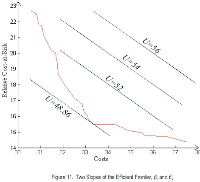
The slope of the left side of the kinked point, , is more steeper slope than that of the right side of the kinked point , . As the consequence of the decrease of Cost-at-Risk in the efficient frontier, the expected cost increases. Compared to the decrease of Cost-at-Risk in the efficient frontier in the left side of the kinked point, the decrease of Cost-at-Risk in right side of the kinked point is followed by a significant increase in the expected cost. Beyond the kinked point, there is no benefit of the increase of the expected cost because it is not compensated by a significant decrease in the exposure of interest rate risk.
5. Government Bond Optimization
Optimum point of the government bond portfolio can be found by using a utility function. When the government has the same preference of risk and cost, it will given by
dRCaR dC
dRCaR dC
Figure 11. Two Slopes of the Efficient Frontier, â1 and â2
For the utility function of U = Cost + Relative Cost-at-Risk, it is the kinked point of 9-10-9-1-1 that minimizes the utility function, the most optimum point for the government if they have the equal preference of cost over risk.
6. Conclusion
Multi-period Cost-at-Risk analysis gives the government a broader perspective in managing its interest rate risk and an opportunity to minimize it by arranging their bond portfolio. In the first years, short-term bonds will yield lower cost but tend to give higher Cost-at-Risk. Higher exposure of Cost-at-Risk can be compensated by choosing long-term bonds in last years because it gives lower Cost-at-Risk and lower NPV of costs compared to issuing them in the first years since the costs will be dispersed 15 years after the bonds are issued (19 until 20 years from present – higher discount factor). Interest rate volatility has a negative relationship with the maturity of the bond (Puhle, 2007).
The interest rates of bonds with long maturity are less volatile than those of short maturity. Therefore, although long-term bonds yield higher NPV of costs, the variance of the costs' NPV (which directly affects the Cost-at-Risk and is the manifest of interest rate risk) can be minimized. If the government chooses the contrary, issuing larger portions of the long-term bonds in the first years then it is inefficient from the Cost-at-Risk perspective, giving them higher costs of debt but not compensated with commensurate decrease on the Cost-at-Risk.
References
Antara Press Office,( July 19th, 2010).
Bolder, David, (2002). A Stochastic Simulation Framework for the Government of Canada's Debt Strategy. Ottawa: Bank of Canada.
Brealey, R., Myers, S. (2003). Corporate Finance: Capital Investment and Valuation. New York: McGraw-Hill.
Cox, J., Ingersoll, J., and Ross, S., (1985). A Theory of the Term Structure of Interest Rates.
Econometrica, 53, pp. 385-408.
Danmarks National bank. (1999). Danish Government Borrowing and Debt . Copenhagen: Danmarks National bank.
De la Grandville, Olivier. (2001). , “Bond Pricing and Portfolio Analysis”, Cambrigde: MIT Press. Hahm, J-H., Kim, J.(2003). Cost-at-Risk and Benchmark Government Debt Portfolio in Korea.
International Economic Journal, 17, pp79-103.
Hull, John C. (1999). Options, Futures, and Other Derivatives. 4th ed., New Jersey: Prentice Hall. Puhle, Michael. (2007). Bond Portfolio Optimization, Doctoral Dissertation, University of Passau. Svoboda, Simona. (2003). Interest Rate Modeling, Hampshire: Palgrave-MacMillan.
Vasicek, O. (1977). An Equilibrium Characterization of the Term Structure of the Interest Rates. Journal of Financial Economics, 5, pp. 177-188.
Zenios, S., Holmer, M., McKendall, R., Vassiadou-Zeniou, C. (1998). Dynamic Models for Fixed-Income Portfolio Management Under Uncertainty. Journal of Economic Dynamics and Control,vol. 22,, pp. 1517-1541.