Normals of the buttery subdivision scheme surfaces
and their applications
P. Shenkmana, N. Dynb, D. Levinb;∗ aI.I.S.R. Ltd., Israel
b
School of Mathematical Sciences, Tel-Aviv University, Ramat-Aviv, 69978 Tel-Aviv, Israel
Received 18 February 1998; received in revised form 23 July 1998
Abstract
The paper presents explicit formulas for calculating normals to surfaces generated by the buttery interpolatory sub-division scheme from a general initial triangulation of control points. Two applications of these formulas are presented: building osets to surfaces generated by the buttery scheme and Gouraud shading of surfaces generated by this scheme as well as shading of their osets. c1999 Elsevier Science B.V. All rights reserved.
Keywords:Triangulation; Subdivision; Buttery scheme; Regular and irregular points; Normals; Osets; Shading
1. Introduction
Subdivision schemes are ecient tools for the fast generation of curves and surfaces from initial control nets. The basic approach to the design of curves and surfaces in computer-aided geometric design consists of using control points {p0
i}i∈I⊂Rs for I⊂Zm; m= 1;2; s= 2;3 dening a control
polygon or a 3D control net together with a smoothing scheme. A subdivision scheme denes recursively a new set of control points {pk
i} at level k from the set at level k−1 for k= 1;2; : : : . Each set of control points at levelk denes a parametric piecewise linear curvepk(t) when t∈⊂R or a parametric piecewise low-degree polynomial surface pk(s; t);(s; t)∈⊂R2. The subdivision
curve or surface is dened as the limit of this sequence when k→ ∞. A subdivision scheme is interpolatory if each set of control points at any level includes all the control points of the previous level.
The buttery interpolatory subdivision scheme [5] is a generalization of the 4-point scheme for curve design to surfaces produced from a general triangulation of control points. The 4-point
∗Corresponding author. E-mail: [email protected].
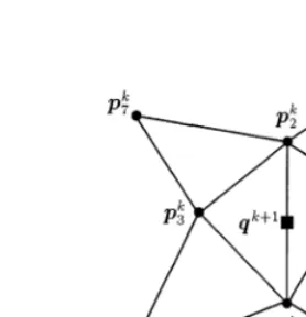
Fig. 1. Conguration of points for the rule for inserting new points in the buttery scheme.
interpolatory subdivision scheme was introduced in [4] and is dened as follows:
(
i=−2 is a set of initial control points. The parameter w serves as a tension parameter
in the sense that decreasing its value to zero is equivalent to tightening the limit curve toward the piecewise linear curve between the initial control points [4].
At each subdivision stage the buttery subdivision scheme transforms each triangular face of the triangulation into four triangular faces which consist of the vertices of the old triangle and three new vertices corresponding to the edges of the old triangle, connected each to the other two and to the vertices of the old edge it corresponds to. The rule for inserting new points is an 8-point rule based on the buttery-like conguration shown in Fig. 1:
qk+1=1
The parameter w serves as a tension parameter in the same sense as the tension parameter in the 4-point scheme.
If we take control points that describe function values over a regular symmetrical three direction mesh, that are constant along one of the directions, then all the new values added at all the stages of the buttery subdivision will be constant along this direction and the scheme reduces to the 4-point scheme along the other two directions [5]. This shows that the buttery scheme is indeed a generalization of the 4-point scheme.
curve dened by the 4-point subdivision process (1) is dierentiable, then at any xed stage m¿0 the tangent vector at the control point pm
i ∈Rs (s= 2;3), corresponding to the parameter value 2−mi, can be evaluated as follows:
p′(2−mi) = 2 m+k
1−4w[
1 2(p
m+k i+1 −p
m+k
i−1)−w(p
m+k i+2 −p
m+k
i−2)] (3)
or with k= 0
p′(2−mi) = 2 m
1−4w[
1 2(p
m
i+1−pmi−1)−w(pim+2−pmi−2)]:
This paper presents similar formulas for the partial derivatives of surfaces generated by the buttery scheme. The formulas were obtained by an analogous local analysis for surfaces. A similar technique for other subdivision schemes was used in [11, 14]. Normals are calculated as vector products of two partial derivatives. These normals are then used in two applications: building osets to surfaces generated by the buttery scheme and Gouraud shading of surfaces generated by this scheme as well as shading of their osets. Formulas for the normals of surfaces generated by a modied version of the buttery scheme are given (without derivation) in [22].
2. Computing normals
The dierential properties of the surface produced by the buttery scheme depend on the degrees of the vertices in the triangulation (the degree of a vertex is the number of edges meeting at the vertex). A vertex of degree 6 is called regular, a vertex of degree other than 6 is called irregular. If all the vertices are regular, the triangulation is termed regular and is topologically equivalent to a three direction grid. A triangulation is irregular if it contains irregular vertices. Since all the new points inserted at each subdivision stage are regular, a regular triangulation remains regular after any number of subdivision stages and an irregular triangulation becomes regular almost everywhere but for neighborhoods of the initial irregular vertices.
2.1. The regular triangulation case
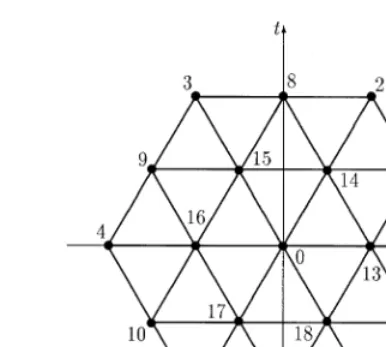
Consider the buttery scheme on a regular triangulation containing only regular control points (of degree 6). This triangulation is topologically equivalent to a regular symmetrical three direction grid with directions (1;0);(1;√3);(1;−√3) (see Fig. 2). It was shown in [10] that for such a triangulation the buttery scheme generates parametric surfaces with C1 components for 0¡w¡1
12.
Let us choose a parameterization in the parameters plane (s; t) such that the parametric points corresponding to the control points together with the connecting edges form a regular 3-direction mesh with edges of length 1 (see Fig. 2). At each stage of the subdivision process new parametric points are inserted at midpoints of old edges in the parameters plane (s; t) forming a new mesh with the same topology but with distances scaled by 1
Fig. 2. A symmetric three direction grid.
Let us investigate the scheme acting on scalar control points representing one component of the vector control points, i.e. the scheme that operates on function valuesf(s; t) over a regular 3-direction mesh in the parameters plane.
Denote by Fk the vector of values (Fk
0; : : : ; F18k)T∈R19 attributed by the buttery scheme to points
in the (s; t) plane with parameters values
(s0+ 2−(m+k)l1; t0+ 2−(m+k)l2); k¿0:
Here (s0; t0) is a xed point on the regular grid generated at xed level m, andl1;l2 are the vectors of
thes-component andt-component, respectively, of the parametric points corresponding to Fk
0; : : : ; F18k,
as depicted in Fig. 2:
l1= (0;2; 1;−1;−2; −1; 1;32; 0;−32;−32; 0; 32;1; 12;−21;−1; −12; 12)T;
l2= (0;0;
√
3;√3; 0;−√3;−√3;√23;√3;√23;−√23;−√3;−√23;0;√23;√23; 0;−√23;−√23)T:
The point F0
0=F0k is inserted at stage m and {Fik}18i=1 are 18 points in its neighborhood at stage
m+k:{Fk
i}12i=1 are located on the outer ring around F00 while {Fik}18i=13 are located on the inner ring
(see Fig. 2). The point (s0; t0) corresponds to the origin in Fig. 2.
Theorem 1. Let w be such that any limit function of the buttery subdivision process (operating on function values over a regular 3-direction grid) is dierentiable at (s0; t0) and let Fk= (F0k; : : : ;
Fk
18)T; s0 andt0 be as above. Then the partial derivatives of the limit function f(s; t)at (s0; t0) are
fs(s0; t0) =c{12w2[2(F1k−F
k
4) + (F
k
2 −F
k
3) + (F
k
6 −F
k
5)]
−6w[(F7k−F9k) + (F12k −F10k)] +(1−4w)[2(Fk
13−F
k
16) + (F
k
14−F
k
15) + (F
k
18−F
k
ft(s0; t0) =c
Proof. The subdivision process in the neighborhood of (s0; t0) can be expressed by the following
A33=
Since the buttery scheme reproduces linear functions (a necessary condition to generate C1
surfaces [3]), the vector e∈R19 with all components equal to 1, and the vectors
l=l1+l2; ||+||¿0;
where l1 and l2 are dened in p. 4, satisfy
Te=e; Tl=12l: (6)
Thus e is an eigenvector of T, corresponding to the eigenvalue 1 and l1 and l2 are eigenvectors,
corresponding to the multiple eigenvalue 12. Let us denote by C3; : : : ;C18 the remaining eigenvectors, corresponding to the eigenvalues 3; : : : ; 18.
Note that the rst row of T is a left eigenvector ofT, corresponding to the eigenvalue 1. Denoting this row of T by r, we get
For general data (9) implies that (7) can hold only if
lim k→∞(2i)
k
In this case
lim k→∞2
m+k(Fk
−Fk
0e) = 2
m(
1l1+2l2): (10)
Comparing (10) and (7) we conclude that
fs(s0; t0) = 2m1; ft(s0; t0) = 2m2: (11)
Let the left eigenvectors of T;u1 andu2, corresponding to the multiple eigenvalue 12, be normalized
such that u1·l1= 1; u1·l2= 0 and u2·l2= 1; u2·l1= 0. Then by (8) and (11)
fs(s0; t0) = 2m1= 2m+ku1·Fk;
ft(s0; t0) = 2m2= 2m+ku2·Fk: (12)
The claim of the theorem follows from (12) and the following explicit form of u1 and u2:
u1=c0(0|q1|q2|q3); u2=c0(0|q4|q5|q6):
Here q1; : : : ;q6 are the following vectors:
q1= 12w2(2;1;−1;−2;−1;1);
q2= 6w(−1;0;1;1;0;−1);
q3= (1−4w)(2;1;−1;−2;−1;1);
q4= 12w2(0;1;1;0;−1;−1);
q5= 2w(−1;−2;−1;1;2;1);
q6= (1−4w)(0;1;1;0;−1;−1);
c0=
1
6(1−6w)(1−4w):
Remark 1. The fact that the buttery scheme is a generalization of the 4-point scheme can help us to verify the previous result. Suppose that the values {Fk
i} are constant along one of the mesh directions. Then it can be easily seen that formulas (4) for the directional derivatives of the functions generated by the buttery scheme along the other two directions reduce to the derivative of the 4-point scheme (3). It is in agreement with the fact that in this case the buttery scheme reduces to the 4-point scheme along these two directions.
Corollary 1. The vectors of partial derivatives of the parametric surface generated by the buttery scheme on a regular triangulation, at the control point pm
0 corresponding to the parameters values
(s0; t0); can be evaluated as follows:
ps(s0; t0) =c{12w2[2(p1m−pm4) + (pm2 −pm3) + (pm6 −p5m)]
−6w[(pm7 −p9m) + (pm12−pm10)]
pt(s0; t0) =c
√
3{12w2[(pm
2 −pm6) + (pm3 −pm5)]
−2w[2(pm
8 −pm11) + (pm7 −p12m) + (pm9 −pm10)]
+(1−4w)[(pm14−p18m) + (p15m −pm17)]};
where the points {pm
i }18i=1 are 18 neighbors of p0m at stage m; corresponding to the parameters
values (s0+ 2−ml1; t0+ 2−ml2) (see their corresponding points in the parameters plane in Fig. 2
where pm
0; : : : ;pm18 are replaced by 0; : : : ;18); s0; t0;l1;l2 are dened as above and
c= 2
m
6(1−6w)(1−4w):
The normal vector to the surface at the point pm
0 is
n= ps(s0; t0)×pt(s0; t0)
kps(s0; t0)×pt(s0; t0)k
:
Proof. This is a direct consequence of Theorem 1 applied to each component of the parametric surface with k= 0.
2.2. The irregular triangulation case
Consider the buttery scheme on an irregular triangulation containing both regular control points (of degree 6) and irregular ones (of degrees other than 6). Since all the new points inserted by the scheme are regular ones, the analysis of the previous subsection applies to most of the surface, excluding neighborhoods of the initial irregular points, where a local analysis is needed.
The technique for calculating the derivatives of a surface produced by the buttery scheme on a
regular triangulationcan be generalized to the case of anirregular triangulation. The main dierence is that the local parameterization near an irregular point depends on the eigenvectors corresponding to the leading eigenvalue smaller than 1 (in absolute value) of the matrix T corresponding to the irregular point. This eigenvalue is not necessarily 1
2 as it is near a regular point. Its value depends
on the tension parameter w and on the degree of the point (the number of edges meeting at the point).
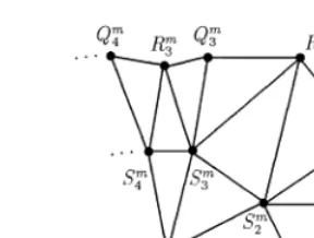
Let us investigate the buttery scheme at stage m near a point Pm, regular or not, of degree n. All the results are valid for regular points, too, as a regular point of degree 6 is a special case of a point of degree n. Assume that the n neighbors of a point Pm are regular (of degree 6). If they are not, then after one subdivision stage (performed locally at the neighborhood of Pm) the new neighbors of Pm+1=Pm will be regular. Following Doo-Sabin construction [2], let us consider 3n points in the neighborhood of Pm: n points located on the inner ring around Pm and 2n their neighbors located on the outer ring. This topology around Pm=Pm+k for k¿0 is preserved at each stage of the subdivision process.
These points at each stage can be classied into three dierent types (see Fig. 3): 1. {Qm
i }ni=1 are the points of the outer ring that belong to the inner ring of stage m−1;
2. {Rm
i }ni=1 are the points of the outer ring that are generated at stage m;
3. {Sm
Fig. 3. Points for calculating rst partial derivatives of the limit functions generated by the buttery scheme in the neighborhood of an irregular point.
Table 1
Ranges ofw sucient for the matrixT to have a correct spectral structure
n 4 5 6 7 8 9 10
w (0, 0.08] (0, 0.10] (0, 0.12] (0, 0.14] [0.07, 0.15] [0.10, 0.16] [0.11, 0.18]
According to this notation, the buttery scheme in the neighborhood of Pm is given by
Pm+1=Pm; Qmi+1=Sim; Rm+1
i =
1 2(S
m
i +S
m
i+1) + 2w(P
m+Rm
i )−w(Q m
i +Q
m i+1+S
m i−1+S
m i+2);
Sim+1=12(Pm+Sim) + 2w(Sim−1+Sim+1)−w(Rmi−1+Rmi +Sim−2+Sim+2);
(13)
where all the indices run from 1 to nand have to be understood modulo n (indices −1;0; n+ 1; n+ 2 stand for n−1; n;1;2; respectively). Eqs. (13) determine the matrix T.
The analysis of the irregular case is deferred for the Appendix, since it is rather technical. Given here are the main results.
Proposition 1. Suppose that w is within the range given in Table 1. Let be the root of maximal absolute value of the cubic equation
3−[12 + 4w(1 + ˆc1−cˆ21)]
2+ [w(2 + ˆc
1) + 6w2(1 + ˆc1−2 ˆc21)]−2w 2(1 + ˆc
1) = 0; (14)
where cˆ1= cos(2=n). Then is the leading eigenvalue smaller than 1 (in absolute value) with
multiplicity 2 of the matrix T; and is a real number. cannot be the leading eigenvalue for
n= 3.
Remark 2. Similar ranges were found for n¿10; too.
Consider the surface produced by the buttery scheme near the pointPmat stagemas a parametric surface. Let us choose a local parameterization such that the points Pm; Qm
1; : : : ; Qnm; Rm1; : : : ; Rmn; S1m
: : : ; Sm
n at stage m correspond to the parameters values
(m−1l
Fig. 4. Parametrization for the buttery scheme in the neighborhood of an irregular point.
where l1;l2∈R3n+1 are linearly independent right eigenvectors of T corresponding to the eigenvalue
. Fig. 4 depicts the points in the parameters plane corresponding to these control points. This choice of parameterization conforms with the regular case when n= 6. At each stage of the subdivision process new points are inserted according to this parameterization forming a new mesh with the same topology but with distances scaled by .
Let us now investigate the scheme operating on real numbers representing one of the components of the control points, i.e. the scheme generating function values f(s; t) over the mesh dened by the chosen parameterization (15).
Theorem 2. Suppose that w is within the ranges given in Table 1 and f(s;t) is a real-valued function; generated by the buttery subdivision process operating on function values over the mesh dened by the parameterization (15). If f(s;t) is dierentiable at (0;0); then
where is dened in Proposition 1 and
c=2
The proof of this result is given in the Appendix.
Remark 3. It is easy to see that the partial derivatives formulas (16) together with the parameteri-zation (15) for n= 6 reduce to those for the regular triangulation (4) (in this case =1
Corollary 2. Assume that the surface produced by the buttery scheme as a parametric surface with the local parameterization (15) at a control point Pm of degree n corresponding to the
parameters values (0;0) is C1. Then the partial derivatives vectors of the surface at Pm can be
evaluated as follows (see Fig. 3) :
ps(0;0) =c0
where is dened in Proposition 1 and
c0=
The unit normal vector to the surface at this point is
n(0;0) = ps(0;0)×pt(0;0)
kps(0;0)×pt(0;0)k :
Proof. This is a direct consequence of Theorem 2 applied to each coordinate of the parametric surface when k= 0.
Remark 4. The above formulas are applicable for a regular or irregular control point Pm with regular neighbors. As previously mentioned; if some of the neighbors are irregular; then one subdivision stage should be performed locally at the neighborhood of Pm producing the new regular neighbors of Pm+1=Pm that are used only for the normal calculation at Pm.
3. Applications
Corollaries 1 and 2 give us explicit formulas for the normals to the limit surface at regular or irregular control points respectively (the formulas are applicable for regular points of degree 6 and for irregular points of degrees 4,5,7,8,9,10, when the tension parameter is within the ranges given in Table 1).
So, at each subdivision level we have a control polyhedron of this level (a piecewise linear interpolant at the control points to the limit surface) with exact normals to the limit surface at the control points. These normals can be used in some applications.
3.1. Gouraud shading
A surface generated by the buttery subdivision scheme can be displayed by shading its control polyhedron at some stage of the subdivision process. The greater is the number of iterations, the closer is the control polyhedron to the limit surface. In constant shading (also known as faceted shading) each triangular face of the polyhedron is shaded with one color intensity depending on the face’s normal. In this case each face is easily distinguished from its neighbors with dierent normals producing a faceted appearance, and many iterations are required to obtain a satisfactory results. Fortunately, with exact surface normals at the polyhedron’s vertices, we can use the intensity interpolation shading also called Gouraud shading [9], when the color intensities of the vertices of each triangle (computed from exact surface normals) are linearly interpolated across the triangle, producing color intensities of its pixels. With this shading model the polyhedron appears like a smooth surface and closer to the limit surface. Note that when shading with a z-buer algorithm, intensities of pixels can be calculated together with their z coordinates which are interpolated in the same way.
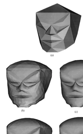
Figs. 5 and 6 show the dierence between constant shading and Gouraud shading. Fig. 5 presents a constant-shaded head-like control polyhedron (a), the same polyhedron after 2 iterations in constant shading (b) and Gouraud shading (c), and after 3 iterations in constant shading (d) and Gouraud shading (e). Fig. 6 presents the same for a cup-like control polyhedron. Note that quadrangular faces seen in the shaded control polyhedrons actually consist of triangles. We can easily see a faceted appearance of the constant-shaded surfaces even after 3 iterations, whereas Gouraud shading after either 2 or 3 iterations looks just like a smooth surface, faces are not distinguished from each other. There is no signicant dierence between 2 and 3 iterations in Gouraud shading.
3.2. Building osets
Oset surfaces are loci of points that lie at a prescribed signed distance from the original surfaces (called generators). Ifr(s; t) is a parametric surface with a unit normal vector n(s; t), then the oset surface at a distanced∈Risr(s; t)+dn(s; t). Hered¿0 means an oset in that side of the generator that is dened by the normal, d¡0 means an oset in the opposite side.
and their osets are recomputed until the distance between the generated oset patch and the gen-erator’s patch at some test points does not dier signicantly from the oset distance. However, a similar algorithm for surfaces generated by the buttery subdivision scheme, that builds approximate osets as surfaces of the same representation, appeared to be inapplicable for several reasons:
• The number of points required to obtain a satisfactory accuracy is too large.
• The accuracy at test points does not guarantee the same accuracy at other points of the segment between two control points (this is true for the above-mentioned algorithms, too).
• The above algorithm generally leads to a control polyhedron for the oset surface with edges that dier signicantly from each other in their length. The buttery subdivision scheme in this situation may produce loops even where the control polyhedron does not form loops.
Thus, another approach is taken. Since oset points of the generator’s control points at each stage of the subdivision process can be quickly calculated in terms of the exact normals, and these oset points are points lying on the exact oset surface, we suggest the following solution. The oset surface can be represented by the generator’s control polyhedron just as the generator itself is. A piecewise linear approximation to the oset surface of any desired accuracy can be obtained from this polyhedron by the following process. First, the buttery subdivision process is carried out up to the appropriate stage producing the new rened set of the generator’s control points. If more accuracy is required in some areas, additional subdivision stages can be performed locally in these areas. Second, the polyhedron that is a piecewise linear approximation to the oset surface is obtained by osetting these control points with the use of the explicit formulas for the normals (Corollaries 1 and 2).
Since vertices of the oset polyhedron are osets of the generator’s control points, normals to the oset surface at these vertices are equal to the normals of the original surface at the corresponding control points. Thus, the approximate osets to surfaces generated by the buttery scheme can be rendered using Gouraud shading in the same way as the original surfaces.
Both exact and approximate oset surfaces may contain singularities such as loops;‘islands’, and more complex self-intersections. Loops occurs at points corresponding to those of the generator with the radius of curvature smaller than the oset distance. ‘Islands’ may occur when the space between parts of the generator surface is too small, more exactly when the distance between the oset of one part of the generator and the other part of it is less than or equal to the oset distance. Detecting and removing such singularities produces the trimmed oset (the locus with the property that each point of it is at a prescribed signed distance d from some point and at a distance d at least from
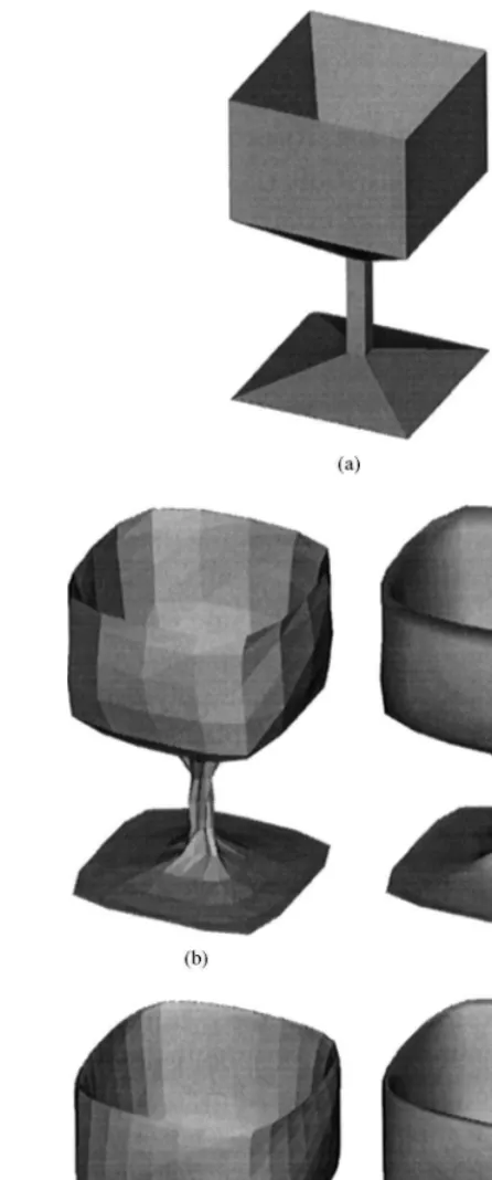
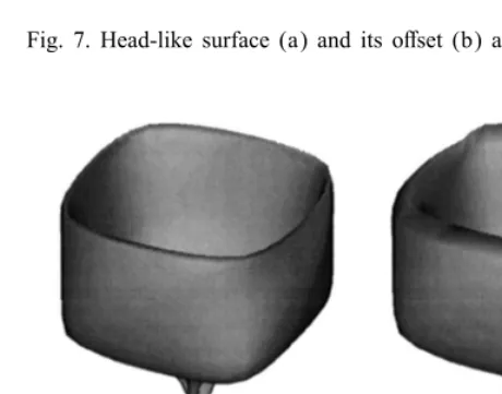
Fig. 7. Head-like surface (a) and its oset (b) after three iterations.
Fig. 8. Cup-like surface (a) and its oset (b) after three iterations.
surfaces can be developed. However, such an algorithm would be much more complicated. Trimming osets of surfaces was investigated by several authors for special cases such as exact osets of twice dierentiable parametric surfaces [1] and approximate osets to general parametric surfaces [21].
Acknowledgements
We thank Gershon Elber for bringing to our attention the Gouraud shading.
Appendix A
The buttery scheme in the neighborhood of Pm given by (13) can be expressed as the following matrix transformation:
where {Aij}3i; j=1 are n×n circulant matrices.
Let us denote the transformation matrix in (A.1) by T. We investigate rst the spectral properties of T.
A circulant matrix
B=
b1 b2 b3 : : : bn−1 bn
bn b1 b2 : : : bn−2 bn−1
bn−1 bn b1 : : : bn−3 bn−2
..
. ... ... . .. ... ...
b3 b4 b5 : : : b1 b2
b2 b3 b4 : : : bn b1
has complex right eigenvectors
wk= (1; k; 2k; : : : ; (n−1)k)T; k= 0;1; : : : ; n−1 (A.2)
and eigenvalues b(k), where b(x) is the polynomial
b(x) = n
X
i=1
determining B, and where
= e’i= e(2i=n):
For the circulant matrices {Aij}3i; j=1 let us denote the determining polynomials by {aij(x)}3i; j=1.
Lemma 1. The matrix T has an eigenvalue 0= 1 with a corresponding right eigenvector C0=e=
(1;1; : : : ;1)T. The other 3n eigenvalues can be calculated as follows:for each k= 0;1; : : : ; n−1 the
Proof. It follows from (13) that the sum of elements of each row of the matrix T is equal to 1. Therefore T has an eigenvalue 1 with an eigenvector e= (1;1; : : : ;1)T. The structure of T implies
that all the remaining eigenvalues are the eigenvalues of the reduced matrix
which consists of circulant blocks with the same eigenvectors wk. Thus the right eigenvectors of T′ can be found as vectors of the form
(wTk|wTk|wTk)T
and the right eigenvectors of T other than e are vectors of the form
This implies that and the eigenvectors of T can be found from (A.4).
Using the explicit form of {aij(x)}3i; j=1 and after some derivations based on (A.4) we arrive at
The detailed proofs of this lemma and Lemma 2 can be found in [19].
Using a similar technique we arrive at
Lemma 2. The left eigenvector of the matrix T corresponding to the eigenvalue 0= 1is the rst
row ofT. The left eigenvectors of the matrixT corresponding to the eigenvalues3k+1; 3k+2; 3k+3;
where wk are dened by (A.2), and where
′
Note that the right and left eigenvectors for k6=12n are not expressed by the formulas in Lemmas 1 and 2, but these eigenvectors are not relevant for our work.
Fig. 9. The case n= 4: (a) graph of absolute values of three roots of the cubic equation (14); (b) graph of
x(w) =|| −maxm=06 ;4;3n−2|m|.
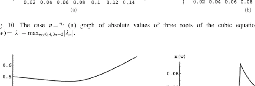
Fig. 10. The case n= 7: (a) graph of absolute values of three roots of the cubic equation (14); (b) graph of
x(w) =|| −maxm=06 ;4;3n−2|m|.
Fig. 11. The case n= 8: (a) graph of absolute values of three roots of the cubic equation (14); (b) graph of
Sucient conditions for C1 continuity and regularity of the limit surface of a subdivision process
near irregular points are given in [17]. The conditions involve the leading eigenvalue of T′ and the characteristic map R27→R2 (dened in [17]) of the subdivision process. The characteristic map
depends only on the eigenvectors corresponding to the leading eigenvalue and the basis-functions of the limit surface. If the leading eigenvalue is a real eigenvalue with multiplicity 2 and if the characteristic map is regular and injective, then the limit surface of the subdivision process is C1 at
each irregular point of degree n, and a regular smooth parametrization exists near such points for almost every initial set of control points.
It was analytically shown in [18] that the above conditions can hold only if the leading eigenvalue is 4=3(n−1)+1 and it is real. It was numerically checked for some values of w that are within the
ranges from Table 1 (sucient for to be both a real number and the leading eigenvalue of T, as we will see below) that the characteristic map is regular and injective. Let us denote 4 by .
Lemma 3. The ranges of the tension parameter w presented in Table 1 are sucient for to be both a real number and the leading eigenvalue of T for n= 4;5; : : : ;10.
Proof. As is the root of maximal absolute value of the cubic equation (14), is real if and only if the root of maximal absolute value of this equation is real. The lemma is proved by checking the graphs of absolute values of three roots of the cubic equation (14) and the graphs of x(w) =|| −
maxm6=0;4;3n−2|m| for n= 3;4; : : : ;10. Some of these graphs (for n= 4;7;8) are presented in Figs. 9–11 (generated with the use of ‘Mathematica’ software). All graphs and the details of the proof can be found in [19].
Suppose that w is within the above-mentioned ranges. As is a real eigenvalue of multiplicity 2 of a real-valued matrix T, we can take l1= Re(C4) and l2= Im(C4) as linearly independent right
eigenvectors andl′
1= Re(C′4) andl2′= Im(C′4) as linearly independent left eigenvectors of the matrixT,
corresponding to the eigenvalue . According to (A.3), (A.7) and (A.2)
l1= (0;cˆ0;cˆ1; : : : ;cˆn−1;|4|cˆ1=2;|4|cˆ3=2; : : : ;|4|cˆ(2n−1)=2; 4cˆ0; 4cˆ1; : : : ; 4cˆn−1)T;
l2= (0;sˆ0;sˆ1; : : : ;sˆn−1;|4|sˆ1=2;|4|sˆ3=2; : : : ;|4|sˆ(2n−1)=2; 4sˆ0; 4sˆ1; : : : ; 4sˆn−1)T;
l′
1 and l2′ are dened like l1 and l2 but with 4′ and ′4 instead of 4 and 4. Here ˆck= cosk’= cos(2k=n); sˆk= sink’= sin(2k=n).
Proof of Theorem 2. The matrix transformation (A.1) implies that
Fk+1=TFk: (A.8)
Now, e is the eigenvector of T, corresponding to the eigenvalue 1, l1 and l2 are those,
corre-sponding to the eigenvalue of multiplicity 2, i.e.,
Te=e; Tl1=l1; Tl2=l2: (A.9)
If the limit function f(s; t) is dierentiable at (0,0), then necessarily (using the parameterization (15))
lim
k→∞
1−(m+k)(Fk−Fk
Denote by ˆC3; : : : ;ˆ
C3n the rest of the eigenvectors of T, except for the three in (A.9). It follows from (A.3) that
This, in view of (A.8) and (A.9), yields
Fk=TkF0=F0
Let us denote by u1 and u2 the left eigenvectors of T, corresponding to the eigenvalue of
mul-tiplicity 2 (linear combinations of l′
1 and l2′) such that u1·l1= 1; u1·l2= 0 and u2·l2= 1; u2·l1= 0.
and note that for arbitrary ’0
(C(’0))2= cos2’0+ cos2(’0+’) +· · ·+ cos2(’0+ (n−1)’)
[1] S. Aomura, T. Uehara, Self-intersection of an oset surface, Comput. Aided Design 22 (1990) 417– 422.
[2] D. Doo, M. Sabin, Behaviour of recursive division surfaces near extraordinary points, Comput. Aided Design 10 (1978) 356 –360.
[3] N. Dyn, D. Levin, Smooth interpolation by bisection algorithms, Approximation Theory 5 (1986) 335–337. [4] N. Dyn, J.A. Gregory, D. Levin, A 4-point interpolatory subdivision scheme for curve design, Comput. Aided Geom.
Design 4 (1987) 257–268.
[5] N. Dyn, J.A. Gregory, D. Levin, A buttery subdivision scheme for surface interpolation with tension control, ACM Trans. Graphics 9 (1990) 160 –169.
[6] R.T. Farouki, Exact oset procedure for simple solids, Comput. Aided Geom. Design 2 (1985) 257–280.
[10] J.A. Gregory, An introduction to bivariate uniform subdivision, in: D.F. Griths, G.A. Watson (Eds.), Numerical Analysis 1991, Pitman Research Notes in Mathematics, Longman Scientic and Technical, New York, 1991, pp. 103–117.
[11] M. Halstead, M. Kass, T. DeRose Ecient, fair interpolation using Catmull–Clark surfaces, SIGGRAPH ’93 Proc. 27 (1993) 35– 44.
[12] J. Hoscheck, Oset curves in the plane, Comput. Aided Design 17 (1985) 77– 82.
[13] Y. Kasas, A subdivision based algorithm for surface=surface intersection, M.Sc. Thesis, Tel-Aviv University, 1990. [14] L. Kobbelt, K. Daubert, H-P. Seidel, Ray tracing of subdivision surfaces, in: G. Drettakis, N. Max (Eds.), Rendering
Techniques ’98, Springer Computer Science, 1998, 69–80.
[15] R.R. Martin, Principal patches for computational geometry, Ph.D. Thesis, Cambridge University, UK, 1982. [16] P. Pottmann, Rational curves and surfaces with rational osets, Comput. Aided Geom. Design 12 (1995) 175–192. [17] U. Reif, A unied approach to subdivision algorithms near extraordinary vertices, Comput. Aided Geom. Design 12
(1995) 153–174.
[18] P. Shenkman, Computing normals and osets of curves and surfaces generated by subdivision schemes, M.Sc. Thesis, Tel-Aviv University, Israel, 1996.
[19] P. Shenkman, N. Dyn, D. Levin, Derivation of normals of the buttery subdivision scheme surfaces at irregular points, Technical report, Tel-Aviv University, Israel, 1998.
[20] W. Tiller, E.G. Hanson, Osets of two-dimensional proles, IEEE Comput. Graph. Appl. 4 (1984) 36 – 46. [21] Y. Wang, Intersection of osets of parametric surfaces, Comput. Aided Geom. Design 13 (1996) 453– 465. [22] D. Zorin, P. Schroder, W. Sweldens, Interpolating subdivision for meshes of arbitrary topology, Computer Graphics