The nite volume method and application in combinations
Zi-Cai Lia;∗, Song Wangb
aDepartment of Applied Mathematics, National Sun Yat-Sen University, Kaohsiung, Taiwan 80424, ROC b
School of Mathematics& Statistics, Curtin University of Technology, CPO Box U1987, Perth 6845, Australia
Received 15 May 1998; received in revised form 30 October 1998
Abstract
In this paper, the conventional nite volume method (FVM) is interpreted as a new kind of Galerkin nite element method (FEM), where the same piecewise linear functions are chosen as in both trial and test spaces, and some specic integration rules are adopted. Error analysis is made for the regular Delaunay triangulation involving obtuse triangles separated, to prove optimal convergence rates of the approximate solutions obtained. The new interpretation makes the FVM analysis much easier because we may bypass verication of the nontrivial Ladyzhenskaya–Babuska–Brezzi (LBB) condition by the Petrov–Galerkin FEM in the existing analysis of FVM. More importantly, the new interpretation and the simple FVM analysis enable us to construct easily the combinations of FVM with other popular numerical methods, such as the nite element method (FEM), the nite dierence method (FDM), the Ritz–Galerkin method (RGM), etc., for solving complicated problems of partial dierential equations (PDE). For example, for solving singularity problems, the combination of RGM–FVM is superior to the combination of RGM–FDM in exibility of arbitrary solution domains, and also superior to the combination of RGM–FEM in substantial saving of CPU time. Since the conservative law of ux may be maintained exactly in the numerical solutions, and since obtuse triangles may be included in the Delaunay triangulation, the FVM and its combinations become very promising for solving elliptic boundary value problems, in particular those where singularity solutions exist and those where the obeying of conservative law is crucial. The numerical examples of combinations of RGM–FVM are given for solving Motz’s problems, to verify the optimal convergence rates. The techniques and analysis of FVM and its combinations can be extended to the convection–diusion problems. Most importantly, an important aspect in this paper is the possibility to include obtuse triangles in the error analysis. c1999 Elsevier Science B.V. All rights reserved.
MSC:65N30; 65N10
Keywords:Elliptic boundary problem; Singularity problem; Combined method; Finite volume method; Delaunay triangulation; Voronoi polygon
∗
Corresponding author.
E-mail address: [email protected] (Z.-C. Li).
1. Introduction
Many numerical approaches have been developed for solving elliptic boundary value problems: the nite element method (FEM) [7] and the nite dierence method (FDM) [10] are most popular. The FEM using triangulation and piecewise low-order polynomials is well suited to arbitrary solution domains and variant coecients. However, the programming of FEM is rather complicated, and demands a great deal of CPU time in formulating the discrete algebraic equations. On the other hand, the classic FDM is simple to form the associated matrix, but dicult to apply for the arbitrary solution domains since the dierence grids are conned themselves to coordinate lines only. There exists the third popular kind of numerical method: the nite volume method (FVM) [38] based on the conservative law in physics. Since the triangular elements may be chosen, the FVM is also applied to rather arbitrary solution domains. Also, the associated matrix of FVM is easy to construct, consumes less CPU time, and has good properties such as positive denite, symmetric, sparse and M-matrix-like [38]. Hence the FVM has the advantages of both FEM and FDM. Moreover, the FVM has a remarkable advantage over FEM and FDM in that it preserves the conservation law exactly in numerical approximations. Hence, the FVM has been widely applied in many engineering and physical problems [23,26,32].
In [38], the triangulation of solution domains was conned to have acute and right triangles. The deep analysis on FVM was developed only in the past decade. Since the associated matrix in FVM is an M-matrix, the error in the maximum norms of numerical solutions can be obtained by the discrete maximum principle (see [32]). This is, indeed, the analytic approach of FDM. The alternative is based on FEM analysis, to give the energy errors of approximate solutions including the solutions and their generalized derivatives.
The dierence equations of FVM are established on the Voronoi polygons of a triangulation [36], which are formed by the perpendicular bisectors of triangle edges. The triangulation may be extended to the Delaunay triangulation which allows obtuse triangles (see [15,29,30]). Some relations between FEM and FVM are explored in [13,36]. The Delaunay triangulation has already been adopted in FVM by Miller and Wang [22–24].
The analysis using FEM approaches was reported rst by Bank and Rose [3] in 1987, and then by Cai [5], Cai et al. [6] and Hackbusch [12]. The Petrov–Galerkin FEM is solicited by choosing the solution space on triangulation and the dierent trial spaces on the Voronoi polygons, also see [22]. The optimal convergence rate O(h) of the errors in the energy norms is reached by proving the inf-sup condition of Ladyzhenskaya–Babuska–Brezzi (the LBB condition) [7]. The improved convergence rate O(h2) can also be achieved by using local uniformity of triangulation [5,6,12].
Although the quadrilaterals are developed for FVM in [16,33], the rectangular elements are often chosen by many authors, such as McCormick [21], Ewing et al. [8], Greenstadt [11] and Miller and Wang [23]. The variants of FVM may be called the box method [3,33], cell discretization [11] and the conservative scheme [38]; all of them are based on the conservative law. Note that triangles in the analysis of [5,6] are limited to being non-obtuse, avoiding the trouble that the circumcenters are located outside the triangles. There seems to exist no analysis so far for the FVM involving obtuse triangles. This paper is devoted to the analysis on FVM for the Delaunay triangulation involving obtuse triangles.
linear functions on the Delaunay triangulation. Interestingly, by using some special integration rules, the discrete dierence schemes obtained are identical to those from the traditional FVM on the Voronoi polygons.
The simple interpretation of FVM as FEM enables us to easily embed FVM into the family of combined methods, in which dierent numerical methods such as FEM, FDM, BEM, etc. are integrated together, to solve a complicated elliptic boundary value problem.
For solving the elliptic boundary problems with singularity problems, we have used the combina-tions in [17–20], in which the RGM is used by means of singular funccombina-tions near the singular points, and the FEM (or FDM) is used for the subdomains with smooth solutions. A further exploration in this paper is to adopt FVM, instead of FEM and FDM, to match RGM. Evidently, the combi-nation of RGM–FVM owns the advantages of both combicombi-nation of RGM–FEM and combicombi-nation of RGM–FDM. Moreover, the new view of FVM as the Galerkin FEM in this paper is also important to eigenvalue and parabolic problems.
We have just noticed that our principal approaches in this paper have been in existence for over seventeen years, see [1,2,14,31], even though they used dierent names and did not indicate explicitly relations to the FVM. In the pioneering work [2,14], approaches similar to Section 2.3 were stated, and they were called the FEM satisfying maximum principle. The dierence schemes obtained also maintain the conservative law; they are, indeed, the FVM called in this paper. In [2,14], only the weakly acute triangles were discussed. The maximum principle is another important physical law, by which the property that the solutions must be nonnegative is maintained. The FVM can produce numerical solutions satisfying both the conservative law and the maximum principle; but the traditional FEM in [7,34] does not. In some physical problems such as convection–diusion problems, both the conservative law and the maximum principle are critical [1,2,9,14,25,31,37,38]. Owing to the convection–diusion problem the FVM becomes a rather independent method (see [1,2,9,14,25 –28,31,37]). Of course, the plentiful achievements of FEM may also be incorporated to the study of FVM. In [1,31], the FVM of weakly acute triangulation is developed for convection– diusion problems, by means of the FEM analysis. Recently, in [9], the combination of FVM–FEM was also developed for nonlinear convection–diusion problems, but with weakly acute type of triangular grids. In [37], analysis of FVM is interpreted as a kind of FEM, also to avoid verication of the LBB condition. However, Vanselow and Scheer [37] invoke nonconforming elements and integration approximation; both are involved in variational crimes (see [34]). In this paper, the FVM interpreted as FEM only with integration approximation may t easily into the family of combined methods in [17–20]. Several combinations in [19] can be extended to combinations of FVM and useful matching techniques may be employed therein.
2. The nite volume method
Let us consider the self-adjoint elliptic equation with the Dirichlet boundary condition
− ▽p▽u+cu=f in ;
u= 0 on ; (2.1)
where is a polygon, =@, the functions c¿0; p¿p0¿0, andp and c are suciently smooth.
For simplicity, only the homogeneous Dirichlet condition is discussed because other boundary condi-tions such as Neumann and Robin condicondi-tions are similar. We will rst discuss the convex polygonal
, and then the concave polygonal in Section 6:2. When is partitioned into acute and right triangles, the FVM can be easily formed (see [38]). In this paper, we consider the Delaunay trian-gulation, where the obtuse triangles are permitted. However, for Neumann and Robin conditions, we should assume that all the circumcenters of triangles are in the closed .
2.1. Delaunay triangulation and Voronoi diagram
A triangulation Th of consists of triangles △i, i.e, =Th =Si△i, and Xh is the set of all
vertices of △i ∈ Th. A triangulation Th is said to be a Delaunay triangulation if for each triangle
△i∈Th, no other vertices in Xh are within its circumcircle (see Fig. 1).
An auxiliary Voronoi diagram (or Dirichlet tessellation) is formed by the perpendicular bisectors of all triangle edges. The Voronoi polygons of the Delaunay triangulation can be dened by
=Sh= N
[
i=1
Si;
where the convex polygons
Si={x∈; |x−xi|¡|x−xj|; xi∈Xh; j6=i}: (2.2)
Eq. (2.2) implies that the ith polygon Si contains all the points in closest to xi.
Now we provide several properties of Delaunay triangles, which will be employed in the FVM and in the error analysis in Sections 3–5.
Property 2.1. For a polygonal ; there exists a Delaunay triangulation.
Property 2.2. The algebraic length of the segment connecting the circumcenters of two neighboring
triangles is nonnegative in a Delaunay triangulation; where two neighboring triangles denote two
connected triangles with common edges.
Property 2.3. The Voronoi polygons associated with a Delaunay triangulation have positive edges
and areas.
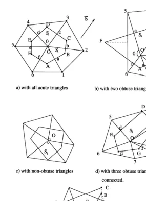
Several dierent cases of Voronoi polygons Si are illustrated in Fig. 2, related to obtuse triangles.
The circumcenters of the acute and obtuse triangles are inside and outside the triangles, respectively. For a right-angled triangle, the circumcenter is just on the hypotenuse.
There may exist a tile Si that contains several obtuse triangles. In Fig. 2d, three obtuse triangles
are connected with the slant edges of the Voronoi polygons, where the largest angle is not located at center O. In Fig. 2e, all four triangles in Si are obtuse, but only two obtuse triangles are connected.
Property 2.4. There exists no Voronoi polygon Si that has all obtuse triangles connected.
Proof of Propositions 2:1–2:4 are either easy or given in [30]. If the acute angles are not located at center O, there may occur for Si all obtuse triangles (see Fig. 2e).
It has been pointed out in [30] that the average number of edges of Voronoi polygons is smaller than six. The Delaunay triangulation is said to be regular if all triangles in a Delaunay triangulation are of regular family of triangulation (see [7,29]). A triangle is said to be regular if its minimal interior angle has a positive lower bound independent of the maximal boundary length h of all triangles. This implies that the ratios of three boundary lengths also have a positive lower bound independent of h. Hence any Voronoi polygon Si of a regular Delaunay triangulation connects nite
number of triangles, and then contains nite edges. Then we write this as a property.
Property 2.5. The number of edges is nite in a Voronoi polygon Si of a regular Delaunay
triangulation.
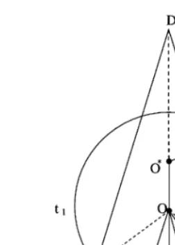
For triangle △ABC in Fig. 3, letOE; OF andOG denote the edges of the perpendicular bisectors between circumcenters O and the midpoints of the boundary edges. We also use OG in Fig. 3 to represent its algebraic length of OG in the sense: usually OG=|OG|¿0, but OG ¡0 if ABC is obtuse and if OG is the distance from the exterior O to the slant edge of △ABC (see Fig. 3). We have the following important property, which is often used in the FVM and its analysis.
Property 2.6. If triangle △ABC in Fig. 3 is regular; then there exists at least two edges with
lengths¿ch;among |OE|;|OF|and|OG|;whereh is the maximal boundary length of△ABC; c is
a positive constant independent of h. Moreover; if △ABC is also obtuse and OG ¡0; then two
Fig. 2. The Voronoi polygons.
Proof. We argue this by contradiction for the obtuse triangle only. Suppose that (see Fig. 3)
|OG|= o(h); |OF|= o(h):
Then we have from the triangle inequality
|GF|6|OG|+|OF|= o(h):
However |GF|=1
2|AC|¿ch due to the regular assumption of △ABC. This contradiction proves the
Fig. 3. The Delaunay triangles with obtuse triangles.
Next consider the obtuse triangle △ABC, in Fig. 3. Assume OG ¡0. Since △OGF is also an obtuse triangle, the slant boundary OF is largest, i.e., |OF|¿|GF|¿ch. Similarly we have
|OE|¿|GE|¿ch.
2.2. Description of the nite volume method
Let the solution domain be partitioned into a regular Delaunay triangulation
=h=
[
i
△i; (2.3)
and also into the corresponding Voronoi polygons
=Sh=
[
i
Si:
Denoting by h the maximum edge length of all △i, we integrate the two sides of (2.1) and use
Green’s formula to obtain
−
I
@Si
pundS+
Z Z
Si
cudS= Z Z
Si
fdS; (2.4)
where un=@u=@n, and n is the outward normal direction to @Si.
To describe the FVM we take as an example the interior vertex i as shown in both Fig. 2a and b with two obtuse triangles. Let ui denote the solution at vertex i, the capitals A; B; : : : ; etc. denote
the circumcenters, and lower cases a; b; : : : ; etc. denote the intersection of the triangle edges and the perpendicular bisectors. Based on Property 2:3, the edge length of the Voronoi polygon Si is
positive. Hence, we have the following approximation: I
@Si
pun=
Z
AB∪BC∪CD∪DE∪EF∪FA
pundS
+|EF|(pun)e+|FA|(pun)f
≈ |AB|pa
u1−u0
|10| +|BC|pb
u2−u0
|20| +|CD|pc
u3−u0
|30|
+|DE|pd
u4−u0
|40| +|EF|pe
u5−u0
|50| +|FA|pf
u6−u0
|60| ; (2.5) where |AB| and |10| are the absolute lengths of AB and 10 respectively. Note that (2.5) is valid for the cases in both Fig. 2a and b involving obtuse triangles.
Since Area(Si)¿0 by Property 2:3
Z Z
Si
cudS ≈c0u0|Si|;
Z Z
Si
fdS ≈f0|Si|; (2.6)
where Si=|Si| is the area of Si. Eqs. (2.4) – (2.6) lead to the linear algebraic equations
Ax=b; (2.7)
where A is positive denite, symmetric, sparse and M-matrix (see [38]), b is a known vector, and x
is the unknown vector with the componentsui at all interior vertices of triangles. Based on Properties
2:2 and 2:3 the Delaunay triangulation guarantees stability of the solutions of (2.7).
The simplicity of evaluating the entries of A as (2.5) is very promising, contrasted to the compli-cated computation in FEM which consumes a great amount of CPU time. Since the obtuse triangles are allowed, the FVM given in this paper may also be suited to more arbitrary shapes of . More-over, Eq. (2.7) also reects the conservation law and the maximum principle in physics. This is particularly attractive to many physical problems. Consequently, the FVM may compete with other methods such as FEM, FDM, etc.
2.3. New view of the nite volume method
The nite volume method can be regarded as the Petrov–Galerkin FEM with dual spaces, where the piecewise linear functions are chosen on a Delaunay triangulation, and the piecewise constants on the Voronoi polygons. Since the LBB condition is not easy to verify, we will invoke the Galerkin FEM, where both the solution and trial functions are chosen to be the same piecewise linear functions on the Delaunay triangulation. Note that the admissible functions chosen below are conforming; but specic rules of integration are used.
Eq. (2.1) can be written in the following weak form: Find the solution u∈H1
0() such that
A(u; v) =f(v); ∀v∈H1
0(); (2.8)
with
A(u; v) = Z Z
(p3u·3v+cuv) dS; (2.9)
f(v) = Z Z
fvdS; (2.10)
where H1
0()(⊂H1()) is the Sobolev space such that
H1 0() =
Let V0
h ⊂H01() be the span of the piecewise linear basis functions constructed on the Delaunay
triangulation h in (2.3). We dene the following FEM with an approximate integration: To seek
˜
The symbols RRc and Rb denote, respectively, the approximations of integrals RR and R by some numerical quadrature rules. However, dierent quadrature rules may be chosen for dierent integrals, in contrast to a uniform rule in the traditional FEM [7]. For the Delaunay triangulation,
ˆ
Let us rst prove an important lemma.
Lemma 2.7. Let lk
i (k = 1;2;3) be the edges between the circumcenter and the vertices of i;
the triangle be split by the edges lk
i into △i =S3k=1△ki; dki be the algebraic distances between
circumcenters Oi and the midpoints of lki; and vi0 the value of v at center Oi. (When △i is obtuse;
Oi 6∈ △i and v0i|at O for v∈Vh0 is the exterior interpolation value of the linear function v in △i:)
Then there exists an equality:
Z Z
whereul andun are; respectively; the tangential and normal derivatives along the outside edges of
i;and
Proof. By applying the Green formula on the triangle △i, we have from (2.1)
When v= 1,
On the other hand,
2
The desired results (2.17) are obtained by subtracting (2.21) from (2.22). This completes the proof of the lemma.
It follows from Lemma 2.7 that Z Z
if other terms on the right-hand side of (2.17) are negligible. A strict error analysis is given later in Theorems 3.3, 3.7 and Eq. (3.44).
Fig. 4. A pair of Delaunay triangles.
12;23 and 31. Hence, Eqs. (2.15) and (2.16) reduce to
ˆ
Ah(u; v) =
X
i 3
X
k=1
( 2 d
Z Z
△k i
pulvldS+
d Z Z
△k i
cuvdS
)
; (2.25)
ˆ
fh(v) =X
i 3
X
k=1
( d Z Z
△k i
fvdS
)
: (2.26)
The FVM described in Section 2.2 can also be derived from (2.12), (2.25) and (2.26), with the help of the special integration rules given below.
We also use △A31 as the algebraic area, where △A31¿0 if the direction of vertices A→3→1 is counter clockwise (Fig. 4a), and otherwise △A31¡0 (Fig. 4b). Note that when△i is obtuse, one
and only one of the sub-triangles △1
i, △2i and △3i has negative area, i.e., △1i =△A31¡0 in Fig.
4b. Hence, we allow the negative △k
i in (2.25) – (2.26). We choose the following approximation of
integrals on △123 (Fig. 4):
3
X
k=1
d Z Z
△k
1
pulvldl= (pulvl)a△A12 + (pulvl)b△A23 + (pulvl)c△A31
=pa
(u2−u1)
|12|
(v2−v1)
|12| △A12 +pb
(u3−u2)
|32|
(v3−v2)
|32| △A23
+pc
(u1−u3)
|13|
(v1−v3)
|13| △A31; (2.27) and
3
X
k=1
d Z Z
△k i
By using fa= 12(f1+f2), we obtain (Fig. 4)
where Ac1a denotes the area of the quadrilateral Ac1a. Similarly, we have
3
expression related to edge 13,
2
Hence, the following form is obtained, explicitly related only to solution v0 in both Fig. 2a and b.
Finally, from (2.25), (2.26), (2.32) – (2.34) we obtain the discrete form of (2.12) with (2.25) and (2.26), written explicitly as those only involving u0 in Fig. 2a and b
0 = ˆA(u; v)−fˆh(v) =· · ·+v0
Obviously, the same algebraic equations (2.7) (see (2.4) – (2.6)) are obtained by noting that v0 is
arbitrary. This gives a new view of the FVM as FEM.
Now, we restate the FVM as follows: To seek ˜uh∈Vh0 such that
Note that the bilinear form in (2.37) is dierent from that in (2.13), based on Lemma 2:7.
3. Error analysis
In Section 2.3, the new interpretation of FVM as the Galerkin FEM enables us to carry out error analysis simply by Theorem 3.3 shown later, because we bypass the nontrivial verication of the LBB condition. The key analysis in this section is Lemma 2.7 leading to the new view on FVM, Lemma 3.2 giving the norm equivalences, and Theorem 3.7 providing error bounds of important approximate integrations. In this section, we conne FVM basically to the weakly acute triangulation, but the analytical approaches will be extended to the Delaunay triangulation involving obtuse triangles, given in Sections 4 and 5.
To derive error bounds of the solutions by FVM, we dene the new norms
The two terms in (3.1) are dened in (2.32) and(2.33) respectively. The Sobolev norms and semi-norms in H1() are dened by
kvkm=kvkm; =
( X
k6m
Z Z
(Dkv)2dS
)1=2
; (3.3)
|v|m=|v|m; =
( X
k=m
Z Z
(Dkv)2dS
)1=2
: (3.4)
Below we shall prove the equivalence between the norms kvkh and kvk1. We use the equivalent
notation “a≍b” to indicate that there exist two positive constants c0 and c1, independent of a and
b, such that
c0a6b6c1a: (3.5)
Lemma 3.1. Let x andy be two real variables;and 066C; where C is independent of x andy.
Then
x2+y2+(x
±y)2
≍x2+y2:
Proof. We have
x2+y2+(x±y)26(1 + 2)(x2+y2)6C(x2+y2) and
x2+y2+(x
±y)2¿x2+y2:
From the denition (3.5), the proof of Lemma 3.1 is completed.
Lemma 3.2. Let h be a regular triangulation in (2:3) with non-obtuse triangles. Then; for the
piecewise linear function space V0
h on h we have
|v|h ≍ |v|1; kvkh≍ kvk1; ∀v∈Vh0: (3.6)
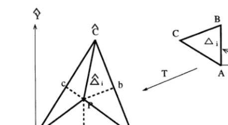
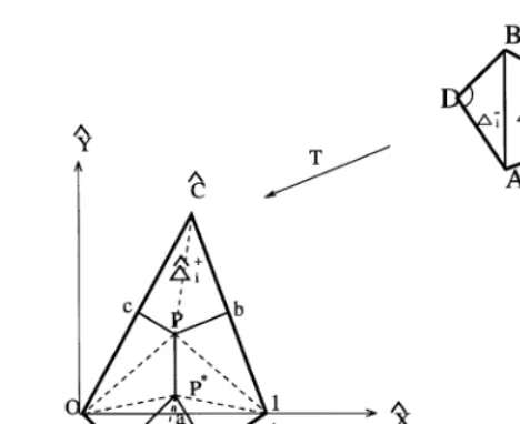
Proof. By a linear conformal transformation T, any triangle △i can be transformed to a reference
triangle ˆ△i (see Fig. 5), where i and ˆi are similar, and the bottom boundary is just on the unit
section of the abscissa ˆX. Such a transformation T is given by xˆ
ˆ
y
=
x
A
yA
+ 1
|AB|
cos sin
−sin cos
x y
: (3.7)
Let
(x; y)→T ( ˆx;yˆ); v(x; y)→T vˆ( ˆx;yˆ): (3.8) From 0¡ p0¡ p ¡ C we have
2
3
X
k=1
d Z Z
△k i
p v2 ldS ≍
3
X
k=1
Z Z
ˆ
△ki
ˆ
v2ld ˆS; ∀v∈V0
Fig. 5. The transformationT from△i to ˆ△i.
Next, denote the linear functions by v=axˆ+byˆ+c in ˆ△i=S3k=1△ˆki of Fig. 5 with arbitrary constants a; b and c, then
3
X
k=1
Z Z
△k i
ˆ
v2ld ˆS= ˆv2x△ PAˆBˆ+ ˆv2l|BˆCˆ △PBˆCˆ + ˆv 2
l|AˆCˆ △ PCˆA;ˆ (3.10)
where the derivatives are given by
ˆ
v2x=a2; vˆ2l|AˆCˆ=
1
|AˆCˆ|2(axˆCˆ+byˆCˆ)
2; (3.11)
ˆ
v2l|BˆCˆ=
1
|BˆCˆ|2(axˆCˆ+byˆCˆ−a)
2: (3.12)
Here (xCˆ; yCˆ) are the coordinates at point ˆC, and|AˆCˆ|=|AˆCˆ|:Triangle ˆ△is regular since ˆ△is similar
to △i. For regular triangle ˆ△ in Fig. 5, the coordinate |yˆCˆ| ≍1, and the edges |AˆCˆ| ≍1; |BˆCˆ| ≍1.
Also based on Property 2:6, at least two of |Pa|, |Pb| and |Pc| are ≍1. By evaluating the areas in (3.10) of Fig. 5, we obtain
=
3
X
k=1
Z Z
ˆ
△ki
ˆ
v2‘d ˆS=a
2
2|Pa|
+1 2
|Pc|
|AˆCˆ|(axˆCˆ +byˆCˆ)
2+ 1
2
|Pb|
|BˆCˆ|(axˆCˆ+byˆCˆ −a)
2: (3.13)
Below we use the Property 2:6 and Lemma 3.1 to show that
1=2=
3
X
k=1
Z Z
ˆ
△ki
ˆ
v2‘d ˆS
!1=2
(3.14)
just denes a two dimensional norm of a and b. Let us consider two cases:
Without loss of generality, suppose |Pb| ≍1. We then choose
x=a; y= (axˆCˆ+byˆCˆ−a); (3.15)
to obtain from Lemma 3.1
=a
2
2|Pa|+ 1 2
|Pb|
|BˆCˆ|y
2+ 1
2
|Pc|
|AˆCˆ|(a+y)
2
≍a2+y2+(a+y)2
≍a2+y2; (3.16)
where =|Pc|=|AˆCˆ| satisfying 066C:
Moreover, we rewrite (3.15) in the matrix-vector form: x
y
=
1 0
ˆ
xC−1 yˆCˆ
a b
: (3.17)
Since the determinant satises
xˆC1−1 yˆ0Cˆ
= ˆyCˆ ≍1:
Thenx(=a) andy can be regarded as two independent variables, and then1=2 is a two dimensional
norm. Since all nite-dimensional norms are equivalent to each other, we have
≍a2+y2 ≍a2+b2: (3.18)
Case II: When |Pa|= o(1), then |Pb| ≍1 and |Pc| ≍ 1 based on Property 2:6. By choosing in Lemma 3.1,
x=axˆCˆ+byˆCˆ; y=axˆCˆ+byˆCˆ−a; a=x−y; (3.19)
we obtain from (3.13)
=1
2(x−y)
2
|Pa|+1 2
|Pc|
|AˆCˆ|x
2+ 1
2
|Pb|
|BˆCˆ|y
2
≍(x−y)2+x2+y2 ≍x2+y2;
where =|Pa|= o(1). Also (3.19) can be written as x
y
=
xˆ
ˆ
C yˆCˆ
ˆ
xCˆ−1 yˆCˆ
a b
;
where the determinant satises
xˆCˆxˆ−Cˆ 1 yyˆˆCCˆˆ
= ˆyCˆ ≍1:
Hence x and y are also two independent variables, so 1=2 also denes a two-dimensional norm,
to lead to
≍x2+y2
For two cases, we conclude
Since all norms in nite dimensions are equivalent to each other, we obtain (also from [7]),
(a2+b2)1=2
≍ |vˆ|1;△ˆi ≍ |v|1;△i: (3.21) Consequently, combining (3.9), (3.20) and(3.21) yields
|v|h=
This is the rst desired result in (3.6). The proof of the second equivalence in (3.6) is similar; this completes the proof of Lemma 3.2.
Now we establish a main theorem for error bounds of the FVM solutions.
Theorem 3.3. Suppose that the Delaunay triangulation is regular;and the following two inequalities
hold:
C0kvk216Aˆh(v; v); ∀v∈Vh0; (3.23)
|A(u; v)|6Ckuk1kvk1; ∀v∈Vh0; (3.24)
where Aˆh(u; v) is dened in (2:37); A(u; v)in(2:9);C is a positive constant independent of h; and
h is the maximal boundary length of regular Delaunay triangles. Then for the solution u˜h of the
FVM(2:36); there exists a bounded constant C independent of h such that
By noting the notations in (2.9) and (2.37), we obtain from Corollary 2.8
Therefore the desired results (3.25) follow from (3.26), (3.27) the triangle inequality, ku−u˜hk16
ku−vk1+kv−u˜hk1. This completes the proof of Theorem 3.3.
Remark 3.4. Let us examine the assumptions (3.24) and (3.23). It is easy to show (3.24) from the
Schwarz inequality; by the Poincare–Friedrichs inequality and Lemma 3.2, we obtain (3.23):
C0kvk216|v|2 ≍ |v|2h6kvk2h6Aˆh(v; v); ∀v∈Vh0:
Below we focus on the estimates on bounds of △Ei(uh; w) in (3.25) given in Theorem 3.7 later,
since the bounds of other terms in (3.25) are easily obtained.
Dene the piecewise constant interpolation u=u|at O in △i. However, when △i is obtuse and
w ∈ V0
h; w=w|at O is obtained from the exterior linear interpolation of w ∈ △i. We have the
following lemma.
Lemma 3.5. Letw ∈ V0
h;and u(=u0i =u|at 0)be the piecewise constant interpolation of u at the
circumcenter O of regular Delaunay△i on h;then
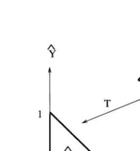
Fig. 6. The linear transformationT from △i to ˆ△i.
Lemma 3.6. Let the conditions in Lemma 3:5 hold. Then
|w−w0i|0; @△i6C
Proof. By noting the linear function w on △i, we have
|w−w0i|0; @△i6Ch|wn|0; @△i6C √
h|wn|1;△i; ∀w∈Vh0: (3.33)
Next, since u is the piecewise constant interpolation of u at the circumcenter of regular Delaunay
△i, we have from the linear transformation T of Fig. 6 (see [7])
|u−u|0; @△i6C
Now we give an important theorem.
Theorem 3.7. Let all conditions in Lemma 3:2 hold and function p be piecewise dierentiable.
whereuh is the piecewise linear interpolant of u on h; andkpk
∗
1;∞; h= maxisup△i{p;|@p=@x|;
|@p=@y|}:
Proof. First letv∈V0
h. Denote by pvn the piecewise constant interpolation ofpvnat the circumcenter
of regular Delaunay △i on h. From Lemma 3.5, we have
From the Schwarz inequality and Lemma 3.6 we obtain Finally by using again the Schwarz inequality, we obtain for v=uh, from (3.36) – (3.37)
In the last step in the above equation, we have used the following bounds,
kuhk16kuhk1+ku−uhk16kuk1+Ch|u|26Ckuk2:
This completes the proof of Theorem 3.7.
Now we turn on estimates of other terms in (3.25). Choose v=uh for the other terms on the
right-hand side of (3.25), where uh is the piecewise linear interpolatory function of u. Then
inf
i. In the last step of the above equation, we have also used the bounds,
Also well as (3.39) – (3.44), we obtain the following theorem.
Theorem 3.8. Letv ∈ H2();and other conditions in Lemma 3:2and Theorem 3:3hold. Then
there exist the error bounds of the solutions by the FVM (2:36)
ku−u˜hk16Ch{kpk
the optimal convergence rate
ku−u˜hk1= O(h) as h→0: (3.46)
Note that the analysis process for the FVM solutions in this section follows the traditional Galerkin FEM analysis in [7], but with a little tedious estimation of integration errors, which is much easier than verifying the LBB condition.
4. Error analysis for Delaunay triangulation involving obtuse triangles separated
A challenge is the analysis for the FVM involving obtuse triangles. We will follow the lines in Sec-tion 3, but rst have to deal with the important task to prove the norm equivalences as in Lemma 3.2, because optimal convergence rates of the FVM solutions below are naturally consequences. Let us state the following important theorem.
Theorem 4.1. Let be partitioned to the regular Delaunay triangulationh involving obtuse
trian-gles separated. There exist the norm equivalences:
|v|h ≍ |v|1; |v|h ≍ kvk1; ∀v∈Vh0; (4.1)
where the norms|v|h andkvkh are dened in(3:1) and(3:2).
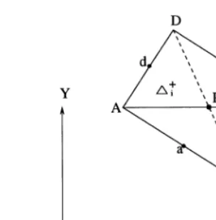
Proof. Since the obtuse triangles are separated, we may consider a pair of Delaunay triangles, where
Fig. 7. The transformationT from △+
i of triangles instead of one triangle in Lemma 3.2. By
the same transformation T in (3.7), we obtain (Fig. 7)
3
By some manipulation, we obtain from Fig. 7
The important fact here is |PP∗|¿0, so that 1=2
k= o(1). There are also two sub-cases:
1. Sub-case I: Both |Pa|= o(1) and |P∗a
|= o(1), then |Pc|;|Pb| ≍1 and |P∗d
| and |P∗e | ≍ 1, based on Property 2:6. We may follow twice the proof of Case II in Lemma 3.2, to obtain (4.5). and II in Lemma 3.2, also to obtain (4.5).
Therefore, for the union of (△+ i ∪ △
−
i ), we conclude from the equivalence of nite dimensional
norms,
Suppose that obtuse triangles and the unions of △+ i ∪ △
Remark 4.2. The proof approaches in Theorem 4.1 may be extended to the Delaunay triangulation
involving multiple (i.e., nite) obtuse triangles connected, as those in Fig. 2d and e, but they fail to give a justication for the case where innite obtuse triangles are connected by their slant edges. The norm equivalence for the Delaunay triangulation involving arbitrary many (i.e., innite) obtuse triangles is still an open and challenging problem.
Fig. 8. The rectangular elements.
Now let us examine the dierent situations in other lemmas and theorems of Sections 2 and 3. Lemma 2.7 holds if the circumcenters Oi can be found outside △i. Note that the linear interpolation
of w ∈ V0
h for circumcenter O outside △i is the exterior linear interpolation. Since △ki may be
negative, we should join (△−i )k∪(△+i )k together in Fig. 7 as done in (4.2). The Schwarz inequality
will operate on the positive union (△+
i )k∪(△
−
i )k as well.
Hence, Theorem 3.3 can be extended to Delaunay triangulation; Lemmas 3.5, 3.6 and Theorem 3.7 are also valid for Delaunay triangulation involving obtuse triangles. In fact, when △i is regular and
obtuse, the distance from the exterior circumcenters O to △i is at most O(h). Hence the exterior
linear interpolation functions will provide the same error order of h as that in Section 3. By the above arguments. Eqs. (3.39) – (3.44) are also valid. We write this conclusion as a theorem.
Theorem 4.3. For regular Delaunay triangulation involving obtuse separated; if all conditions in
Theorem 3:8 hold. Then there also exist the bounds (3:25) and (3:45). Moreover; ifu ∈ H2();
f∈H1(); and kpk∗
1;∞; h andkck1;∞; h are bounded;then
ku−u˜hk1= O(h):
5. Application in combinations
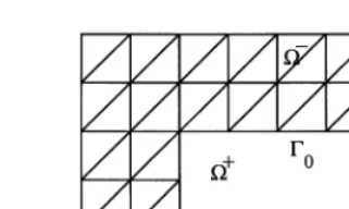
5.1. Rectangular elements
Consider FVM in the case when is split into rectangles i. Hence FVM with the rectangles
may lead to the FDM in [10,17]. The rectangle i in Fig. 8 has the edge lengths h and k. We may
develop the variant of FVM which includes both triangles and rectangles. We will here derive the dierence equations of FVM, based on the new interpretation in Section 2.3. For implicitness, split
i into two right triangles △+i ∪ △
−
i , which belong to Delaunay triangles. The two circumcenters of
△+
i and △
−
Since the degenerate triangle △PAC=0, there exists no contribution of integrals along the diagonal
AC. From (2.36) (see Fig. 8)
3
X
k=1
[
Z Z
(△+
i)k∪(△
−
i )k
2pulvldS
= 2pa
(uB−uA)(vB−vA)
h2 △PAB+ 2pc
(uD−uC)(vD−vC)
h2 △PCD
+2pd
(uA−uD)(vA−vD)
k2 △PDA+ 2pb
(uC−uB)(vC−vB)
k2 △PBC
=1 2
k
h[pa(uB−uA)(vB−vA) +pc(uD−uC)(vD−vC)]
+ h
k[pb(uC−uB)(vC−vB) +pd(uD−uA)(vD−vA)]
;
because △PAB=△PBC=△PDA=△PCD=hk=4: Similarly, we have
3
X
k=1
[
Z Z
(△+
i)k∪(△−i )k
cuvdS=1
2(cAuAvA+cBuBvB)△PAB
+1
2(cBuBvB+cCuCvC)△PBC+ 1
2(cAuAvA+cDuDvD)△PDA +1
2(cDuDvD+cCuCvC)△PCD =hk
4 {cAuAvA+cBuBvB+cCuCvC+cDuDvD}; and
3
X
k=1
[
Z Z
(△+
i)k∪(△−i )k
fvdS= hk
4 {fAvA+fBvB+fCvC+fDvD}: The same dierence schemes as in [10,17] are obtained.
The application to rectangles implies that the FVM may include the rectangular elements whose edges may not be parallel to the coordinate axes. Since the FDM falls into the frame work of the new FVM in this paper, with the Delaunay triangulation including pairs of right triangles as in Fig. 8, we obtain immediately a combination of FDM–FVM, written as the following theorem.
Theorem 5.1. Let be partitioned into regular Delaunay triangles and right triangles in pairs;and
all the conditions in Theorem 4:3 hold. Then the error bounds of solutions from the FVM; i.e.; the
combination of FDM–FVM; also have the optimal convergence rate
ku−u˜hk1= O(h):
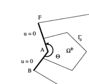
5.2. Combinations of the RGM–FVM for singularity problems
Fig. 9. A partition onfor combinations of RGM–FVM.
that a reentrant angle exists in. We split by 0 into + and
−
, where+ contains the concave
corner point (see Fig. 9). For simplicity, consider the Poisson equation with the Dirichlet condition:
− △u=f; on ;
u= 0; on ; (5.1)
where f= 0 in +. Hence the particular solutions in + are found as
u+=
∞
X
i=1
airisini; (5.2)
where ai are the expansion coecients, and (r; ) are the polar coordinates with origin A. Then
i=i= ¡1 if =“BAF ¿. The admissible functions are chosen as
v+=v
1 in
−
;
v+= L
X
i=1
airisini in +;
(5.3)
where v1 is the piecewise linear functions on the regular Delaunay triangulation of −. We assume
that there are obtuse triangles in −
, but their circumcenters are all in −. The Ritz–Galerkin method(RGM) and the FVM are used in + and −
, respectively. Since the admissible functions (5.3) are not continuous on 0,
v+
6
=v−
on 0; (5.4)
by following [19] we may enforce the following direct constraint conditions for the admissible functions in (5.3) at all nodes Zk of the Delaunay triangles on 0:
v+(Zk) =v
−
Fig. 10. Partition of Motz’s problem with MS = 2.
Denote by V0h the space of the admissible functions (5.3) satisfying v| = 0 and (5.5). We express the nonconforming combination of RGM–FVM: To seek ˆuh∈V
0
h such that
Ah( ˆuh; v) = ˆfh(v); ∀v∈V 0
h; (5.6)
where
ˆ
Ah( ˆuh; v) =
Z Z
+
3u·3vdS+X
i 3
X
k=1
d Z Z
△k i
2ulvldS: (5.7)
Dene the norm
kvkH= (kvk21;++kvk2h)1=2; (5.8)
where kvkh in − is dened by (3.1). The analysis of the combinations (5.6) may follow [19], to
obtain the optimal convergence rates
ku−uˆhkH = O(h); (5.9)
where the number of terms L in (5.3) is suitably chosen as L= O(lnh).
6. Numerical experiments for Motz’s problems
In this section, numerical experiments are carried out to verify the optimal convergence rates O(h) made in Sections 3–5. Let us consider the typical Motz problem (see Fig. 10):
u=@
2u
@x2 +
@2u
@y2 = 0 in; (6.1)
u|x¡0∧y=0= 0; u|x=1= 500; (6.2)
@u @y
y=1
=
@u @y
x¿0∧y=0
=
@u @x
x=−1
where is a rectangle (−16x61, 06y61). The origin (0;0) is a singular point where the solution behaviour is u = O(r1=2) as r → 0 because of the intersection of the Neumann and Dirichlet
conditions.
Divide by 0 into + and−. The subdomain+ is chosen as a smaller rectangle (−126x612,
06y61
2). Also the subdomain
−
is again split into uniform right triangles shown in Fig. 10. The admissible functions are chosen as:
v=
where ˜D‘ are unknown coecients, and (r; ) are the polar coordinates with origin (0,0).
Besides the nonconforming combination in Section 5.2, other combinations are obtained by fol-lowing [19,20],
h is the space of (6.4) satisfying the homogeneous Dirichlet
conditions of (6.2). We employ in (6.5) the additional integrals on 0 to couple v+ and u
− Five combinations of RGM–FVM result from (6.6):
(I) Penalty combination: (Pc¿0; == 0);
(II) Simplied hybrid combination: (Pc= 0; = 1 and = 0);
(III) Combination I: (Pc¿0; = 0 and = 1);
(IV) Combination II: (Pc¿0; = 1 and = 0);
(V) Symmetric combination: (Pc¿0; ==12):
Optimal convergence O(h) of the solutions can be produced by following the analysis of [19]. Let MS denote the uniform dierence division number along BD, where h= 1=(2×MS). Based on the good matching between L + 1 (the total number of basis functions used) and MS given in [19], we will choose
MS = 2 and L + 1 = 4 : MS = 4;6 and L + 1 = 5 : MS = 8 and L + 1 = 6: (6.8) Numerical solutions are conducted by the six combinations of RGM–FVM; and their error norms and the approximate coecients are provided in Tables 1–5 where other error norms are dened by
Table 1
Error norms by nonconforming, penalty and simplied hybrid combinations of RGM–FVM
Methods Nonconf. Penalty Simpf. hybrid
Divisions max kk0; kkH max kk0; kkH max kk0; kkH
MS = 2
L + 1 = 4 2.59 1.16 21.7 10.8 3.15 24.1 3.72 1.21 21.1
MS = 4
L + 1 = 5 0.722 0.289 10.5 2.60 0.769 11.1 0.976 0.305 10.4
MS = 6
L + 1 = 5 0.366 0.131 6.94 1.18 0.345 7.20 0.439 0.136 6.91
MS = 8
L + 1 = 6 0.214 0.074 5.19 0.624 0.194 5.34 0.240 0.076 5.18
Table 2
Error norms by Combinations I, II and symmetric combination of RGM–FVM withPc= 10 and= 2
Comb. I II Symmetric
Divisions max kk0; kkH max kk0; kkH max kk0; kkH
MS = 2
L + 1 = 4 3.34 1.17 21.7 3.37 1.17 21.7 3.37 1.17 21.7
MS = 4
L + 1 = 5 0.943 0.293 10.5 0.945 0.293 10.5 0.945 0.293 10.5
MS = 6
L + 1 = 5 0.451 0.132 6.94 0.453 0.132 6.94 0.453 0.132 6.94
MS = 8
L + 1 = 6 0.282 0.075 5.19 0.283 0.075 5.19 0.282 0.075 5.19
Table 3
Error norms by the nonconforming combination of RGM–FVM withh=1 8
Divisions FVM MS = 7 MS = 6 MS = 5 MS = 4 MS = 3 MS = 2 MS = 1 only L + 1 = 3 L + 1 = 4 L + 1 = 4 L + 1 = 5 L + 1 = 6 L + 1 = 7 L + 1 = 8
max 36.5 2.29 1.93 1.15 0.722 0.644 0.670 0.702
kk0; 8.50 0.481 0.447 0.355 0.289 0.258 0.238 0.201
kkH 58.2 19.1 14.7 12.1 10.5 9.03 7.56 5.66
Con. Num. 218 13153 3170 203 185 233 454 1608
where =u−u˜h. Only the error curves of the solutions by symmetric combination are depicted in
Fig. 11; those for other combinations are similar. It is easy to see from Fig. 11 and the data in Tables 1, 2, 4 and 5 that
Table 4
The leading approximate coecients by the nonconforming combinations of RGM–FVM
Coes. D˜0 D˜1 D˜2 D˜3 D˜4 D˜5
MS = 2
L + 1 = 4 399.449 86.731 14.199 −17.700 / /
MS = 4
L + 1 = 5 400.888 87.404 16.393 −10.919 2.623 /
MS = 6
L + 1 = 5 400.040 87.638 16.782 −9.350 1.949 1.032
MS = 8
L + 1 = 6 401.094 87.647 16.965 −8.791 1.721 0.716
True 401.162 87.656 17.238 −8.071 1.440 0.331
Table 5
The leading approximate coecients ˜D0 by penalty combination, simplied hybrid combination, combinations I, II and
symmetric combination
Comb. Penal. Simpl. I II Symm.
Coes. D˜0 D˜0 D˜0 D˜0 D˜0
MS = 2
L + 1 = 4 399.035 401.582 399.443 399.473 399.439
MS = 4
L + 1 = 5 400.868 401.260 400.876 401.878 400.874
MS = 6
L + 1 = 5 401.037 401.208 401.033 401.033 401.323
MS = 8
L + 1 = 6 401.093 401.188 401.089 401.089 401.089
kk0;= O(h2); max = O(h2
−); (6.11)
|D0−D˜0|= O(h2); |D1−D˜1|= O(h2); (6.12)
whereDi and ˜Di are the true and approximate coecients respectively. Note that Eq. (6.10) coincides
with the theoretical results made in Sections 3–5, and the empirical relations in (6.11) and (6.12) are also optimal.
We may change the size of the subdomain +, to obtain in Table 3 the error norms and
con-dition numbers of the associated matrix, which results from the nonconforming combinations of RGM–FVM. Let BE in Fig. 10 be divided into 8 uniform sections, i.e., h=1
8. Also, MS denotes the
division number along BD. Table 3 lists the results for dierent MS value. It can be seen in Table 3 that that MS = 4 and L+ 1 = 5 are benecial owing to small errors and a small condition number. This implies that the size of + in Fig. 10 is a good choice, which has been chosen as a standard
Fig. 11. The error curves of kkH, kk0; and max by symmetric combination of RGM–FVM withPc= 10 and= 2.
7. Concluding remarks
Although basic ideas and approaches of FVM as FEM in this paper can be found in earlier litera-ture [1,2,14,31], the contributions of this paper lies in analysis of the FVM possibly involving obtuse triangles, to achieve the optimal convergence rates. Moreover, the FVM is applied to combinations so that the FVM may be integrated with other popular numerical methods, such as FEM, FDM, BEM, RGM, etc. (see [19]). To close this paper, let us point out the novelties in this paper:
(1) Based on Lemma 2.7, the FVM can be interpreted as a special kind of Galerkin FEM, in which the solution and trial spaces are the same, but dierent rules of integration approximations are chosen. Theorem 3.7 is a new contribution to yield the error bounds resulting from Lemma 2.7, and to lead to the optimal convergence rate O(h) of the FVM solutions.
(2) The new view of FVM in this paper is simpler than the traditional view as the Petro-Galerkin FEM. The price for avoiding the LBB condition is to establish the norm equivalences, and to solicit the integration rules, where a fair easy evaluation of integration errors is needed.
to nite (i.e., multiple) obtuse triangles connected, which may t in most applications (see those in Fig. 2). The norm equivalence as (4.1) for general cases of Delaunay triangulation involving innite obtuse triangles connected is still an open and challenging problem.
(4) The FVM using the Delaunay triangulation is exible in application for arbitrary solution domains. Because the FVM reserves the conservative law and the maximum principle exactly in numerical solutions so that FVM may compete with FEM and FDM. In fact, the FVM has been applied in many physical and engineering problems, e.g., the singularly perturbed problems [1,2,9,14,23,25,27,31,32,37].
(5) The new interpretation of FVM in this paper is important to integrate FVM into the combined methods. Since FVM is a kind of Galerkin FEM, the combination of FEM–FVM is straightforward. Moreover, in Sections 5.1 and 5.2, combination of FDM–FVM and combination of RGM–FVM are easily established.
(6) Combinations of RGM–FVM is signicant for solving singularity problems. The numerical results of Motz’s problem in Section 6 show that the optimal convergence rates O(h) have been obtained. The theoretical analysis may follow directly from combinations of RGM–FEM in the recent book [19] and this paper.
(7) The new view of FVM as the Galerkin FEM in this paper is also important to eigenvalue and parabolic problems. Take the parabolic problem as an example. If the space and time discretization are chosen as in this paper and Thomee [35], respectively, we may design the dierence schemes to maintain exactly the conservative law even for larget. Some numerical reports of parabolic problems by FVM are given in [4], where the conservative law on the total liquid volume is crucial.
Acknowledgements
We are very grateful to an anonymous reviewer for his=her careful reading, many thoughtful comments, valuable suggestions and kindly providing Refs. [1,2,9,14,31]. This work was supported in part by research grants received from the Natural Scientic Councils of Taiwan and Australia.
References
[1] L. Angermann, Numerical solution of second-order elliptic equations on plane domains, RAIRO Model. Math. Anal. Numer. 25 (2) (1991) 169 –191, Addendum ibidem 27 (1) (1993) 1–7.
[2] K. Baba, M. Tabata, On a conservative upwind nite element scheme for convective diusion equations, RAIRO Model. Math. Anal. Numer. 15 (1) (1981) 3–25.
[3] R.E. Bank, D.J. Rose, Some error estimates for the box method, SIAM. J. Numer. Anal. 24 (1987) 777–787. [4] T.D. Bui, Z.C. Li, N.V. Nguyen, Numerical simulation of liquid redistribution in permeable media involving
hysteresis, Math. Comput. Modeling 28 (1998) 81–103.
[5] Z. Cai, On the nite volume method, Numer. Math. 58 (1991) 713–735.
[6] Z. Cai, J. Mandel, S. McCormick, The nite volume element method for diusion equations on general triangulation, SIAM. J. Numer. Anal. 28 (1991) 392–402.
[7] P.G. Ciarlet, Basic error estimates for elliptic problems, in: P.G. Ciarlet, J.L. Lions (Eds.), Finite Element Methods (Part I), North-Holland, Amsterdam, 1991, pp. 17–351.
[9] M. Feistauer, J. Felcman, M. Luk’acov’a-Medvid’ova’, On the convergence of a combined nite volume-nite element method for nonlinear convection-diusion problems, Numer. Meth. PDE 13 (2) (1997) 163–190.
[10] S.K. Godunov, V.S. Ryabenkii, Dierence Schemes, North-Holland, Amsterdam, 1987.
[11] J. Greenstadt, The cell discretization algorithm for elliptic partial dierential equations, SIAM, J. Sci. Statist. Comput. 3 (1982) 261–288.
[12] W. Hackbusch, On rst and second order box scheme, Computing 41 (1989) 277–296.
[13] S.R. Idelsohn, E. Onate, Finite volume and nite elements: two ‘good friends’, Int. J. Numer. Meth. Eng. 37 (1994) 3323–3341.
[14] T. Ikeda, Maximum Principle in Finite Element Models for Convection-Diusion Phenomena, North-Holland, Amsterdam, 1983.
[15] M. Junger, G. Reinelt, D. Zepf, Computing correct Delaunay triangulation, Computing 47 (1991) 43–49.
[16] A. Lahrmann, An element formulation for the classical nite dierence and nite volume method applied to arbitrary shaped domains, Int. J. Numer. Meth. Eng. 35 (1992) 893–913.
[17] Z.C. Li, Combination of Ritz-Galerkin and nite dierence methods, Int. J. Numer. Meth. Eng. 39 (1996) 1839–1857. [18] Z.C. Li, Penalty combinations of Ritz-Galerkin and nite dierence methods for singularity problems, J. Comput.
Appl. Math. 481 (1997) 1–17.
[19] Z.C. Li, Combined Methods for Elliptic Equations with Singularities, Interfaces and Innities, Kluwer, Amsterdam, 1998.
[20] Z.C. Li, T.D. Bui, Coupling techniques for matching dierent methods in solving singularity problems, Computing 45 (1990) 311–319.
[21] S.F. McCormick, Multilevel Adaptive Methods for Partial Dierential Equations, SIAM, Philadelphia, 1989. [22] J.J.H. Miller, S. Wang, A triangular mixed nite element for the stationary semi-conductor device equations, Math.
Modelling Numer. Anal. 25 (1991) 441–463.
[23] J.J.H. Miller, S. Wang, An exponentially tted nite volume method for the numerical solution of 2D unsteady incompressible ow problems, J. Comput. Phys. 115 (1994) 56–64.
[24] J.J.H. Miller, S. Wang, A tetrahedral mixed nite element for the stationary semi-conductor continuity equations, SIAM J. Numer. Anal. 31 (1994) 196–216.
[25] L.D. Mishev, Finite volume methods on Voronoi meshes, Numer. Meth. PDE 14 (1998) 193–212.
[26] K.W. Morton, Finite volume method, in: D.G. Griths, G.A. Watson (Eds.), Numerical Analysis, Longman, New York, 1995.
[27] K.W. Morton, Numerical Solution of Convection-Diusion Problems, Chapman & Hall, London, 1996.
[28] K.W. Morton, M. Stynes, An analysis of the cell vertex method, Math. Mode l Anal. Nume r. 28 (1994) 699–724. [29] J. Pach (Ed.), New Trends in Discrete and Computational Geometry, Springer, Berlin, 1993, pp. 39.
[30] F.P. Preperata, M.I. Shamos, Computation Geometry, An Introduction, Springer, New York, 1985, pp. 204 –225. [31] U. Risch, An upwind nite element method for singularly perturbed elliptic problems and local estimates in the
L∞-norm, RAIRO Model. Math. Anal. Numer. 24 (2) (1990) 235–264.
[32] H.G. Roos, M. Stynes, L. Tobiska, Numerical Methods for Singularly Perturbed Dierential Equations, Convection-Diusion and Flow Problems, Springer, Berlin, 1996.
[33] T. Schmidt, Box scheme on quadrilateral meshes, Computing 51 (1993) 271–292.
[34] G. Strang, G. J. Fix, An Analysis of the Finite Element Method, Prentice-Hall, Englewood Clis, New York, 1973. [35] V. Thomee, Galerkin Finite Element Methods for Parabolic Problems, Springer, Berlin, 1997.
[36] R. Vanselow, Relation between FEM and FVM applied to the Poisson equation, Computing 57 (1996) 93–104. [37] R. Vanselow, H.P. Scheer, Convergence analysis of a nite volume method via a new nonconforming nite element
method, Numer. Meth. PDE. 14 (1998) 213–231.