Directory UMM :Data Elmu:jurnal:J-a:Journal of Computational And Applied Mathematics:Vol105.Issue1-2.1999:

Perturbations of Laguerre–Hahn linear functionals

F. Marcellana;∗_{, E. Prianes}b

a_{Departamento de Matematicas, Escuela Politecnica Superior, Universidad Carlos III de Madrid, Butarque 15,}

28911, Leganes, Madrid, Spain

b

E.U.I.T.I Virgen de la Paloma, Universidad Politecnica de Madrid, Francos Rodriguez 106, 28039, Madrid, Spain Received 15 September 1997; received in revised form 29 May 1998

Dedicated to Professor Haakon Waadeland on the occasion of his 70th birthday

Abstract

In this paper we shall make some perturbations in a Laguerre–Hahn linear functional, such as the addition of a Dirac Delta or the left multiplication by a polynomial. We shall study that these transformations carried out on Laguerre– Hahn linear functionals originate new Laguerre–Hahn linear functionals. We shall also analyze the class of the resulting functional. c1999 Elsevier Science B.V. All rights reserved.

MSC:42C05

Keywords:Orthogonal polynomial; Quasi-denite linear functional; Recurrence relation; Stieltjes function; Laguerre– Hahn polynomial

1. Introduction

Modications by means of Dirac deltas have been considered by several authors from dierent point of view. In 1940 Krall [12] obtained three new classes of polynomials orthogonal with respect to measures which are not absolutely continuous with respect to the Lebesgue measure; the resulting polynomials satisfy a fourth-order linear dierential equation. Nevai [17] considered the addition of nitely many mass points to a positive measure and he studied the asymptotic behavior of the corresponding orthogonal polynomials. In [13], Maroni and Marcellan were interested in the analysis of modications of semiclassical functionals by adjoining arbitrary masses at any point of the real line. In that paper necessary and sucient conditions for the quasi-deniteness of the modied functional have been given.

∗_{Corresponding author.}

E-mail address: pacomarc@ing.uc3m.es (F. Marcellan).

More recently, in [3, 4], a generalization of the Laguerre classical polynomials has been treated, by adding a derivative of a Dirac delta in the point z= 0. In particular, the hypergeometric character of these new polynomials is showed (see also [6]).

Our aim is to analyze how the Laguerre–Hahn character for the perturbed linear functionals is preserved as well as to determine the class of such a functional (see [1, 14, 18]).

The structure of the paper is as follows: Section 2 contains some introductory results and notations concerning linear functionals. Section 3 is devoted to the characterization of the Laguerre–Hahn linear functionals and the denition of the concept of class. In Section 4 a modication of a Laguerre–Hahn linear functional is carried out by adding a Dirac delta, studying the modication of the order of the class of the new Laguerre–Hahn functional obtained in such a way. In Section 5 we carried out the study of the linear functional U_{, fullling (x−c)}U₌V_{, where} V _{is a Laguerre–Hahn linear} functional, (see [11, 15]), as well as the order of the class of the involved functionals.

The modications mentioned in Sections 4 and 5 have been carried out in the rst kind associated functional for the classical ones, by studying the modication of the order of the class and showing the equations which the new functional satises, as well as the Riccati dierential equation which fulls the corresponding Stieltjes function.

2. Preliminaries and notations

Let U _{be a linear functional on the linear space P of polynomials with complex coecients and} let S(U_{)(z) be its Stieltjes function dened by}

S(U_{)(z) =−}X

n¿0 U_n

zn+1;

whereU_n=hU_{; x}n_{i; n¿0, are the moments ofUandh·;·imeans the duality bracket. By a convention,}

we will suppose that U_{0= 1.} Let P′

be the algebraic dual space of P and the linear space generated by {Dn_}

n¿0, where

Dn _{means the nth derivative of Dirac delta in the origin.}

We consider the isomorphism F_{:→P given as follows (see [16]).}

For U₌X

n¿0

U_n(−1)

n

n! D

n_{; F(U)(z) =}X

n¿0 U_nzn_:

Then,

S(U_{)(z) =−z}−1_F(U)(z−1_):

We introduce

hpU_{; qi=h}U_{; pqi for every polynomialq(z):}

Furthermore, we dene

(U_{p)(z) =}

n

X

m=0

n

X

j=m ajUj−m

!

zm_{; p(z) =} n

X

j=0

and

(0p)(z) =

p(z)−p(0)

z :

Thus, S(pU_{)(z) =p(z)S(}U_{)(z) + (}U_{0p)(z), where p(z) is a polynomial.}

We dene the functional x−1_{U and the product of two linear functionals in the following way:}

hx−1_{U; pi=hU;}

0pi; hUV; pi=hU;Vpi: Then it is straightforward to prove that

(i) x(x−1_{U) =U;} (ii) x−1_{(xU) =U−U}

0;

(iii) x−2_(x2_{U) =x}−1_(x−1_{U) =U−U}

0+U1D:

Remark. We shall use the z variable for all those equations where the Stieltjes function appears and the x variable in the rest of the equations.

Denition 2.1. A linear functional U _{is said to be a quasi-denite or regular (see [9]) functional if} there exists a sequence of monic orthogonal polynomials (MOPS), {Pn}n¿0 with respect to U, i.e., it satises

(i) Pn(x) =xn+ lower degree terms.

(ii) hU_{; P}

nPmi=knnm; kn 6= 0; n= 0;1;2; : : : .

A MOPS {Pn}n¿0 with respect to a quasi-denite linear functional satises the following three-term recurrence relation:

Pn+2(x) = (x−n+1)Pn+1(x)−n+1Pn(x); n¿0; P0(x) = 1; P1(x) =x−0

with n6= 0; n¿0 and 0= 1 =hU; P02i.

Proposition 2.1. A linear functional U _{is quasi-denite if and only if}

n(U) = det[Ui+j]ni; j=0 6= 0;

for all n¿0.

Denition 2.2. Let {Pn}n¿0 be a MOPS with respect to a quasi-denite functionalU. The sequence {P(1)

n }n¿0 dened by

P(1)

n (x) =

U_;Pn+1(x)−Pn+1()

x−

; n¿0

is called the associated sequence of rst kind for the sequence {Pn}n¿0.

Remark. hU_{;·i means the action of} U _{over the polynomial on the -variable.}

We shall note by U(1) _{the normalized functional, [U}(1)

Theorem 2.1. Let U _{be a linear functional. Then}

1U(1)=−x2U−1:

In a general way, the associated sequence of rth kind r = 1;2;3; : : : ;{P(r)

n }n¿0 is dened by the recurrence relation

P_n(₊₂r)(x) = (x−n+r+1)Pn(+1r)(x)−n+r+1Pn(r)(x); n¿0; P₁(r)(x) =x−r; P0(r)(x) = 1:

This corresponds to a shifted perturbation in the coecients of the three-term recurrence relation. We give the following previous results (see [8, 14, 16] for a more comprehensive approach).

Lemma 2.1. For p; q∈P and for U_;V_∈P′

; we have (i) x−1_{(pU) +hU;}

0pi=p(x−1U); (ii) q(U_0p)−U_{0(qp) =−0[(p}U_)q]; (iii) 0(Up) =U(0p);

(iv) U_{(pq) = (p}U_)q+xq(U_0p); (v) p(UV_{) = (p}V₎U_+x(V_0p)U_:

In terms of the Stieltjes functions:

Lemma 2.2. For p∈P and for U_;V_∈P′_{; we have}

(i) S′

(U_{)(z) =S(D}U_)(z);

(ii) S(UV_{)(z) =−zS(}U_)(z)S(V_)(z); (iii) S(x−1_{U)(z) = (1=z)S(U)(z);} (iv) 1

z(U0p)(z) =−

1

z2S(hU; 0pi)(1_z) + (U20p)(z):

3. The Laguerre–Hahn class

Denition 3.1 (Alaya [1]). A linear functionalU_{on the linear spaceP is said to be of the Laguerre–} Hahn class if its Stieltjes function satises a Riccati equation

(z)S′

(U_{)(z) =B(z)S}2₍U_{)(z) +C(z)S(}U_{)(z) +D(z);}

where (z); B(z) and C(z) are polynomials with complex coecients, and

D(z) =−[(DU_{)0](z) + (}U_0C)(z)−(U22

0B)(z); (z)6= 0: (1)

Remark. When B(z) = 0, the Stieltjes function satises a linear dierential equation(z)S′_{(U)(z) =} C(z)S(U_{)(z)+D(z) and the corresponding polynomials are called ane Laguerre–Hahn polynomials.} More precisely, they are the semiclassical polynomials (see [5, 16]).

Theorem 3.1 (Bouakkaz [7], Dini and Maroni [10] and Maroni [16]). LetU_{be a quasi-denite and}

normalized linear functional [(U_{)0=1]and let {Pn}n¿0 be the corresponding MOPS. The following}

statements are equivalent:

(i) U _{is a Laguerre–Hahn functional.}

(ii) U _{veries the functional equation D[}U_{] +} U_+B(x−1_U2_{) = 0; where ; B; and C are}

the polynomials dened in (1); and (x) =−[′

(x) +C(x)]: (2)

(iii) U _{satises the functional equation D[x}U_{] + (x −)}U_+BU2_{= 0 with the additional}

condition hU_{; i+h}U2_;

0Bi= 0 where ; and B are the polynomials dened in (ii). (iv) Each polynomial Pn; n¿0; veries the so-called structural relation

(x)P′

n+1(x)−B(x)P (1)

n (x) = n+d

X

=n−s

n; P(x); n¿s+ 1;

where and B are the polynomials dened in (i) and {P(1)

n }n¿0 is the sequence of associated

orthogonal polynomials of rst kind relative to {Pn}n¿0; where t= deg; p = deg ¿1; r = degB; s= max(p−1; d−2) and d= max(t; r).

3.1. Determination of the order of the class

In the characterization (ii), we must notice that there does not exist uniqueness in the represen-tation. In fact, it is enough to multiply by any polynomial both sides of the equation. On the other hand, uniqueness is obtained by imposing a minimality condition as we will discuss below.

If U _{satises the equation D[}U_{] +} U_+B(x−1_U2_{) = 0, multiplying it by a polynomial q(x), U} satises D[∗_{U] +} ∗_U+B∗_(x−1_U2_{) = 0, where} ∗_=q; ∗_=q

−q′ _{and B}∗_=qB.

We shall associate to U _{the set of nonnegative numbers h(}U_{) ={max(p−1; d−2)}, being}

d= max(t; r), where t= deg∗_{, p= deg} ∗ _{and r= degB}∗_{, among all the possible choices of} ∗_, ∗ _{and B}∗ _{(whenever the quasi-deniteness is preserved).}

Denition 3.3 (Bouakkaz [7]). The class of the Laguerre–Hahn functional U _{is the minimum of}

h(U_).

Theorem 3.2 (Marcellan and Prianes [14] and Prianes [18]). LetU _{be a quasi-denite linear}

func-tional verifying D[U_{] +} U_+B(x−1_U2_{) = 0 where ; and B are the polynomials introduced}

in Theorem 3:1. We dene d= max(t; r)and s= max(p−1; d−2). The Laguerre–Hahn functional

U _{is said to be of class s if and only if}

Y

a∈Z

{|hU_{; ai+h}U2_{; 0Ba)i|+|ra|+|sa|} 6= 0;}

where Z is the set of zeros of (x). The polynomials a; a and Ba as well as the numbers ra

and sa are dened by the expressions

(x) = (x−a)a(x);

Let us establish an equivalent result to Theorem 3.2, where the condition about the class will be given in terms of the polynomials B, C and D dened in (1), using the Stieltjes function.

Corollary 3.1. Let U _{be a quasi-denite linear functional of Laguerre–Hahn class verifying (2).}

A necessary and sucient condition for U _{to be of class s is}

Y

a∈Z

{|B(a)|+|C(a)|+|D(a)|} 6= 0

i.e.; the polynomials ; B; C; and D are coprime.

4. Modication by a Dirac Delta

Proposition 4.1 (Alaya [2], Marcellan and Prianes [13] and Prianes [18]). Let U _{be a Laguerre–}

Hahn linear functional and let and c be complex arbitrary numbers with6= 0.Then;U₌U₊

c

is a Laguerre–Hahn linear functional.

Proof. Let U _{be a Laguerre–Hahn functional fullling (2). Substituting} U _by U _{−c in this} equation, we have

D(U_{) +} U_+B(x−1_U2_)−D(

c)− c−2B[x −1_(U

c)] +2B(x −12

c) = 0: (3)

On the other hand,

hB[x−1_(U

c)]; p(x)i=hU; c(x0Bp)i=hB(x−c)

−1_{U; pi: (4)}

From this B[x−1_(U

c)] =B(x−c)−1U.

Analogously,

hB(x−12

c); p(x)i= lim_x→c

_{(B(x)p(x)−B(0)p(0)}

x−c

=hB′

(c)c−B(c) ′ c; pi

from where

B(x−12

c) =B ′

(c)c−B(c) ′

c: (5)

In a similar way, we obtain

D(c) =(c) ′

c and c= (c)c: (6)

Substituting (4) – (6) in (3),

D(U_{) + [ −2B(x−c)}−1_]U+B(x−1_U2_{) =[(c) +B(c)]}′

c+[ (c)−B ′

(c)]c: (7)

Multiplying (7) by (x−c) and taking into account that (x−c)′

c=−c and (x−c)c= 0, D[(x−c)U_{] + [(x−c) −−2B]}U_+B(x−c)(x−1_U2_{) =−[(c) +B(c)]}

c: (8)

We shall distinguish two situations,

(i) (c) +B(c) = 0, U _{is a Laguerre–Hahn functional, fullling the equation}

(ii) (c) +B(c)6= 0. Then, multiplying (8) by (x−c)

D[(x−c)2_{U] + (x−c)[(x−c) −2−2B]U+ (x−c)}2_B(x−1_U2_{) = 0}

and the proposition holds.

Remark. cp(x) =c[xp(x)], (see [10]). The proof of the proposition can also be carried out with

the help of the Stieltjes function in the following way:

Let S=S(U_{)(z) be the Stieltjes function corresponding to} U_{. This function veries}

(z)S′

=B(z)S2_{+C(z)S+D(z): (9)}

Let S=S(U_{)(z) be the corresponding Stieltjes function for} U_. From hU_{; x}n_i=hU+

c; xni=Un+cn, n¿0, it follows that S=S+=(z−c).

Substituting in (9),

(z−c)2_S′_{= (z−c)}2_BS2_{+ (z−c)[2B+ (z−c)C]S}

+ [+2B+(z−c)C+ (z−c)2D]: (10)

In Proposition 4.4, where we shall study the order of the class of the functional U_{, we shall see if} the condition (c) +B(c) = 0 is fullled, Eq. (10) is reducible and we can divide by (z−c). So (z−c)S′ _{= (z−c)BS}2_{+ [2B+ (z−c)C]S+ [}

c+2Bc+C+ (z−c)D] holds. This agrees

with the results obtained in the proof of Proposition 4.1 using the functional equations.

4.1. Determination of the order of the class

In the following, let us suppose that U _{is a Laguerre–Hahn linear functional of class s.}

Proposition 4.2. LetU _{be a Laguerre–Hahn linear functional of class s;and} U₌U₊

c; 6= 0.

Then U _{is a Laguerre–Hahn linear functional of class s such that s−2}6s6s+ 2.

Proof. We shall use the following notation:

(x) =

s+2

X

i=0

dixi; (x) = s+1

X

i=0

cixi and B(x) = s+2

X

i=0

bixi: (11)

Let D(∗_U

) + ∗_U

+B∗

(x−1_U2_{) = 0 be the equation which fulls U where}

∗

= (x−c)2; ∗

= (x−c)[(x−c) −2−2B] and B∗

= (x−c)2B: (12)

Then deg∗

=t∗

6s+ 4, deg ∗

=p∗

6s+ 3, and degB∗

=r∗

6s+ 4.

Thus d∗_{= max(t}∗_{; r}∗₎

6s+ 4 and s= max(p∗_{−1; d}∗₋₂₎

6s+ 2.

On the other hand, since U₌U_{−c, then s}6s+ 2.

Proposition 4.3. Let U _{be a Laguerre–Hahn functional satisfying Eq. (12). Then for every zero}

Proof. Following Theorem 3.2, we shall write

where the polynomials ; B; C and D are dened in (1).

Proof. We shall use the following notation:

c; i(z) = (z−c)c;(i+1)(z) +tc;(i+1); c;0=;

Bc; i(z) = (z−c)Bc;(i+1)(z) +sc;(i+1); Bc;0=B;

Cc; i(z) = (z−c)Cc;(i+1)(z) +qc;(i+1); Cc;0=C;

Dc; i(z) = (z−c)Dc;(i+1)(z) +pc;(i+1); Dc;0=D:

If (c) +B(c) = 0 holds, the previous equation is divisible by (z−c) and thus the order of the class of U _{decreases in one unit. In fact,}

(z−c)S′_{= (z−c)BS}2_{+ [2B+ (z−c)C)]S+ [}

c;1+2Bc;1+C+ (z−c)D]

and then s=s+ 1: If B(c) = 0 and [c;1+Bc;1+C](c) = 0 this is equivalent to B(c) = 0 and

B′_{(c) +}′_{(c) +C(c) = 0. Thus the previous equation can be divided by (z}

−c) and the class of U _decreases.

S′_=BS2_{+ [2B}

c;1+C]S+ [c;2+2Bc;2+Cc;1+D] and then s=s: Assume (c) =B(c) = 0 (conditions already satised); [2Bc;1+C](c) = 0 and

[c;2+2Bc;2+Cc;1+D](c) = 0 ⇔ 2B

′

(c) +C(c) = 0 and

1 2

2_B′′

(c) + 1 2

′′

(c) +C′

(c) +D(c) = 0:

Then the class of U _decreases.

c;1S′=Bc;1S 2

+ [Bc;2+Cc;1]S+ [c;3+2Bc;3+Cc;2+Dc;1]; s=s−1: Finally,

c;1(c) = 0;

Bc;1(c) = 0;

[2Bc;2+Cc;1](c) = 0;

[c;3+2Bc;3+Cc;2+Dc;1](c) = 0;

then

′

(c) = 0; B′

(c) = 0 (already required)

B′′

(c) +C′

(c) = 0; 2

3!B

′′′

(c) + 3!

′′′

(c) + 2C

′′

(c) +D′

(c) = 0:

S satises

c;2S′=Bc;2S 2

+ [2Bc;3+Cc;2]S+ [c;4+2Bc;4+Cc;3+Dc;2]: Thus, s=s−2.

This result is a more complete description than the presented in [1], Theorem 4:1:5.

4.2. Examples

In the next examples we shall describe the equations which U₌U(1)₊

c satises where U(1)

is the associated functional of the rst kind for the classical polynomials, as well as the Riccati equations which the corresponding Stieltjes function, S(z) =S(U_{)(z), satises.}

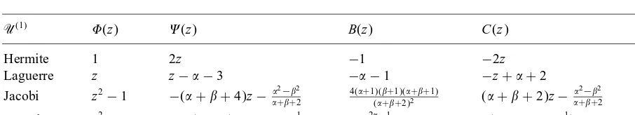
Table 1

U(1) _{(z) (z) B(z) C(z) D(z)}

Hermite 1 2z −1 −2z −2

Laguerre z z−−3 −−1 −z++ 2 −1

Jacobi z2_{−1 −(++ 4)z−}2−2 ++2

4(+1)(+1)(++1)

(++2)2 (++ 2)z−

2−2

++2 ++ 3

Bessel z2 −2[(+ 1)z+ 1−−1_{] −} 2−1

2(2+1) 2(z+ 1−

−1_{) 2+ 1}

The polynomials; ; B; C andD are obtained from the following table (according to Denition 3.1. and Theorem 3.1):

4.3. Hermite polynomials

Let U(1) _{be the linear functional corresponding to the associated polynomials of the rst kind for} the Hermite polynomials and U₌U(1)₊

c, 6= 0.

(i) If 6= 1, (c) +B(c)6= 0. U _{fulls the equation}

D[(x−c)2U_{] + 2(x−c)[(x−c)x+−1]}U_−(x−c)2_(x−1_U2_{) = 0:}

The class of the functional U _{is s= 2 and S(z) satises the equation}

(z−c)2_S′_=−(z−c)2_S2_{+ [−2z}3_{+ 4cz}2_−2(+c2_{)z+ 2c]S}

+ [−2(1 +)z2+ 2c(2 +)z+−2−2c2]:

(ii) If = 1, (c) +B(c) = 0. Since B(c)6= 0, U _{satises the equation}

D[(x−c)U_{] + [2(x−c)x+ 1]}U_−(x−c)(x−1_U2_{) = 0:}

The class of the functional U _{is s= 1 and S(z) veries the equation}

(z−c)S′_=−(z−c)S2_{−2[(z−c)z+ 1]S−2(2z+c):}

4.4. Laguerre polynomials

Let U(1) _{be the linear functional corresponding to the associated polynomials of the rst kind for} the Laguerre polynomials and U₌U(1)₊

c; 6= 0.

(i) If c6=(+ 1) then (c) +B(c)6= 0. U _{fulls the equation}

D[x(x−c)2_{U] + (x−c)[(x−−3)(x−c) + 2(+ 1)−2x]U}

−(+ 1)(x−c)2_(x−1_U2_{) = 0:}

The class of the functional U _{is s= 2 and S(z) satises the equation}

z(z−c)2S′_{=−(+ 1)(z−c)}2_S2_{+ (z−c)[−2(+ 1) + (−z++ 2)(z−c)]S}

(ii) If c=(+ 1); (c) +B(c) = 0, but B(c) =−(+ 1)6= 0; ( 6=−1). Then U _{fulls the} equation

D[x(x−c)U_{] + [2c−(x−c)(−x++ 2)]}U_{−(+ 1)(x−c)(x}−1_U2_{) = 0:} The class of the functional U _{is s= 1 and S(z) satises the equation}

z(z−c)S′_{=−(+ 1)(z−c)S}2_{+ [(z−c)(−z++ 2)−2c]S}

+ _3c

+ 1+

(−z+)c

+ 1 −(z−c)

:

4.5. Jacobi polynomials

Let U(1) _{be the linear functional corresponding to the associated polynomials of the rst kind for} the Jacobi polynomials and U₌U(1)₊

c; 6= 0.

(i) If

6= (1−c

2_{)(++ 3)(++ 2)}2 4(+ 1)(+ 1)(++ 1) ;

then (c) +B(c)6= 0 and s= 2. S and U _{satisfy, respectively,}

(z−c)2(z2−1)S′_{= (z−c)}24(+ 1)(+ 1)(++ 1)

(++ 3)(++ 2)2 S 2

+24(+ 1)(+ 1)(++ 1)

(++ 3)(++ 2)2

+ (z−c) 

2

4(+ 1)(+ 1)(++ 1) (z−c)(++ 3)(++ 2)2

+ (z−c) "

(++ 2)z− 2₋2

(++ 2) #

S

+(z2−1) +(z−c) "

(++ 2)z− 2₋2

(++ 2) #

+ (z−c)2(++ 3);

D[(x−c)2(x2−1)U_{] + (x−c)}24(+ 1)(+ 1)(++ 1) (++ 3)(++ 2)2 (x

−1_U2₎

+ (x−c) "

(x−c) "

−(++ 4)x+ 2₋2

(++ 2) #

−2−(x2−1) #

U_{= 0:}

(ii) If

=(1−c

2_{)(++ 3)(++ 2)}2 4(+ 1)(+ 1)(++ 1) ;

then (c) +B(c) = 0 begin B(c)6= 0 (+=−1 leads to the semiclassical case), and s= 1: S

and U _{satisfy, respectively,}

(z−c)2(z2−1)S′_{= (z−c)}4(+ 1)(+ 1)(++ 1)

(++ 3)(++ 2)2 S 2

+(1−c

Let U(1) _{be the linear functional corresponding to the associated polynomials of the rst kind for} the Jacobi polynomials and U₌U(1)₊ semiclassical case), and s= 1. S and U _{satisfy, respectively,}

D[x(x−c)U_{] + [−(2x−c) + 2c}2_{−2(x−c)(+ 1)x+ 1−}−1_)]U

+ (x−c) (1−2)

2_{(2+ 1)}(x

−1_U2_{) = 0:}

5. Study of the functional U _{such that (x−c)}U₌V_{, and c∈ C, where the} V _{is a}

Laguerre–Hahn functional

Proposition 5.1. LetU _andV _{be two linear functionals related by (x−c)}U₌V_{. Then if} V _is

a Laguerre–Hahn functional; U _{is also a Laguerre–Hahn functional and conversely.}

Proof. Let V _{be a Laguerre–Hahn functional such that the corresponding Stieltjes function S =}

S(V_{)(z) satises the equation}

S′

=BS2_{+CS+D: (13)}

Let S(z) =S(U_{)(z) be the Stieltjes function relative to the functional} U_{. From}

V

n=hV; xni=Un+1−cUn

we get S(z) = (1=)[(z−c)S(z) + 1]. Substituting in (13) we obtain

(z−c)S′_{= (z−c)}2_BS2_{+ [−+ 2(z−c)B+(z−c)C]S+ [B+C+}2_{D]: (14)}

Moreover, U _{satises the equation}

D[(x−c)U_{] + (x−c)[ −2B]}U_{+ (x−c)}2_B(x−1_U2_{) = 0 (15)} with =−′

−C.

Conversely, from the relation betweenS andS we deduce that ifU _{is a Laguerre–Hahn functional,} i.e., S veries the Riccati equation

·S′_{=B S}2_{+C S+D;}

then V_{= (1=)(x −c)}U _{is also a Laguerre–Hahn functional and for the corresponding Stieltjes} function S=S(V_{)(z) the equation}

(z−c)S′

=2BS2+ [−2B+(z−c)C+]S+ [−+B−(z−c)C+ (z−c)2D];

holds.

Furthermore, the functional U _{satises the distributional equation}

D[(x−c)V_{] +[2B+ (x−c) ]}V₊2_B(x−1_V2_{) = 0 (16)}

with =−(′+C).

5.1. Determination of the order of the class

In the following, we will assume that V _{is a Laguerre–Hahn functional of class s.}

Proof. Let ; and B be as in Proposition 4.2 and let D[∗_{U)] +} ∗_U+B∗_(x−1_U2_{) = 0 be the} equation which fulls U _where ∗

=(x−c); ∗

On the other hand, if U _{is a Laguerre–Hahn functional of class s such that}

D[U_{] +} U_+B(x−1_U2_{) = 0; =−(}′_{+C) then V satises the equation}

D[V_{] +} V_+B(x−1_V2_{) = 0; where =(x−c); =[2B+ (x−c) ]; B=}2_B; and deg=t6s+ 3; deg =p6s+ 2; degB∗_=r

6s+ 2.

Thus d= max(t; r)6s+ 3 and s= max(p−1; d−2)6s+ 1.

Proposition 5.3. LetU _{be a Laguerre–Hahn functional satisfying Eq. (15). For every zeroa of}

∗_{=(x−c)dierent from c;Eq.(14)is irreducible.}

where the polynomials; B; C andD are dened in(13).

Proof. We will use the same notation as in Proposition 4.4. If (c)6= 0, S(z) =S(U_{)(z) satises Eq. (14). Then s=s+ 2.}

If (c) = 0 and B(c) +C(c) +2_{D(c) = 0, the previous equation is divisible by (z−c). Thus.}

S′= (z−c)BS2+ [−c;1+ 2B+C]S+ [Bc;1+Cc;1+2Dc;1] and s=s+ 1: If −c;1(c) + 2B(c) +C(c) = 0 and Bc;1(c) +Cc;1(c) +2Dc;1(c) = 0, then

−′

(c) + 2B(c) +C(c) = 0 and B′

(c) +C′

(c) +2D′

(c) = 0:

Dividing by (z−c),

c;1S′=BS 2

+ [−c;2+ 2Bc;1+Cc;1]S+ [Bc;2+Cc;2+2Dc;2] and thens=s:

If      

    

c;1= 0⇒

′

(c) = 0; B(c) = 0;

(−c;2+ 2Bc;1+Cc;1)(c) = 0⇒ −

2

′′

(c) + 2B′

(c) +C′

(c) = 0;

(Bc;2+Cc;2+2Dc;2)(c) = 0⇒B

′′

(c) +C′′

(c) +2_D′′

(c) = 0;

we can divide again by (z−c). So,

c;2S′=Bc;1S 2

+ [−c;3+ 2Bc;2+Cc;2]S+ [Bc;3+Cc;3+2Dc;3] and s=s−1: This result gives a more descriptive analysis than that presented in [1], Lemma 4:2:6.

5.2. Examples

In these examples we shall describe the equations which U _{satises, when (x−c)}U₌V _and V _{is the associated functional of the rst kind for the classical polynomials, as well as the Riccati} equation which satises the corresponding Stieltjes function S(z) =S(U_)(z).

BecauseV _{is a Laguerre–Hahn functional, it fulls a distributional dierential equation andS(z)=}

S(U(1)_{)(z), a Riccati equation.}

The polynomials ; ; B; C and D are obtained from the Table 1.

5.3. Hermite polynomials

(c)6= 0⇒U _{fulls the equation}

D[(x−c)U_{] + 2(x−c)(x+ 1)}U_−(x−c)2_(x−1_U2_{) = 0:}

The class s of the linear functional U _{is s= 2. S(z) satises the equation}

(z−c)S′_=−(z−c)2_S2_{−[+ 2(z−c)(z+ 1)]S−[1 + 2z+ 2}2_]:

5.4. Laguerre polynomials

(i) If c6= 0; (c)= 0 and6 s= 2. U _{and S(z) satisfy, respectively,}

z(z−c)S′_{=−(+ 1)(z−c)}2_S2_{−[z+ 2(+ 1)(z−c) +(z−−2)(z−c)]S}

+ [−2−(+ 1) +(−z++ 2)]:

(ii) If c= 0 and B(c) +C(c) +2_{D(c) =−(+ 1) +(+ 2)−}2 _{6= 0, then s= 2.} Moreover,

D[x2U_{] +x[(x−−3) + 2(+ 1)]}U_{−(+ 1)x}2_(x−1_U2_{) = 0;}

z2S′_{=−(+ 1)z}2_S2_{+ [−z−2(+ 1)z+z(−z++ 2)]S}

+ [−(+ 1) +(−z++ 2)−2_]:

(iii) If c= 0; B(c) +C(c) +2_{D(c) =−(+ 1) +(+ 2)−}2_{= 0 and}

−′

(c) + 2B(c) +C(c) =−−2(+ 1) +(+ 2)6= 0:

Thus s= 1. Furthermore,

D[xU_{] + [2(+ 1)−(−x++ 2)]}U_{−(+ 1)x(x}−1_U2_{) = 0;}

zS′_{=−(+ 1)zS}2_{+ [−−2(+ 1) +(−z++ 2)]S−:}

(iv) If c= 0; B(c) +C(c) +2_{D(c) =−(+ 1) +(+ 2)−}2_{= 0}

−′

(c) + 2B(c) +C(c) =−−2(+ 1) +(+ 2) = 0;

B′

(c) +C′

(c) +2D′

(c) =−6= 0:

Then s= 1. (= 0 is excluded because of the quasi-deniteness condition). U _{and S(z) satisfy,} respectively,

D[xU_{] +(x−1)}U_{−(+ 1)x(x}−1_U2_{) = 0;}

zS′_{=−(+ 1)zS}2_−zS−:

5.5. Jacobi polynomials

(i) If c6=±1; (c) =c2_{−16= 0. Then s= 2.} Moreover,

D[(x−c)2(x2−1)U_{] + (x−c)}

"

"

−(++ 4)x+ 2₋2

(++ 2) #

−8(+ 1)(+ 1)(++ 1)

(++ 3)(++ 2)2

+ (x−c)24(+ 1)(+ 1)(++ 1) (++ 3)(++ 2)2 (x

(ii) If c= 0 andB(c) +C(c) +2_{D(c) = (−2(−1)=}2_{(2+ 1)) + 2(1−}−1_{) +}2_{(2+ 1)6= 0,} then s= 2.

D[x3U_]−2x

₂₍₋₁₎

2_{(2+ 1)}+[(+ 1)x+ 1−

−1_]U−x2 2(−1)

2_{(2+ 1)}(x

−1_U2_{) = 0;}

z3S′_=−z2 2(−1) 2_{(2+ 1)}S

2 +

2z(z+ 1−−1_)−z2_−2z 2(−1)

2_{(2+ 1)}

S

+

− 2(−1)

2_{(2+ 1)}+ 2(z+ 1−

−1_{) +}2_{(2+ 1):}

(iii) If c= 0; B(c) +C(c) +2_{D(c) = 0, and −}′_{(c) + 2B(c) +C(c) =}

−2(2(−1)=2₍₂₊ 1)) + 2(1−−1_{)6= 0, thus s= 1,}

D[x2U_]−

₋₄₍₋₁₎

2_{(2+ 1)} +[(2+ 1)x+ 2−2

−1_]

U_−x 2(−1)

2_{(2+ 1)}(x

−1_U2_{) = 0;}

z2S′_=−z 2(−1) 2_{(2+ 1)}S

2 +

2(z+ 1−−1_)−z− 4(−1)

2_{(2+ 1)}

S+ 2:

(iv) If c= 0; B(c) +C(c) +2_{D(c) = 0; −}′_{(c) + 2B(c) +C(c) = 0, and B}′_{(c) +C}′_{(c) +} 2_D′

(c) = 26= 0, then s= 1,

D[x2_{U]−[x(2+ 1)]U−x} 2(−1)

2_{(2+ 1)}(x

−1_U2_{) = 0;}

z2_S′_=−z 2(−1) 2_{(2+ 1)}S

2

+z(2+ 1)S+ 2:

Acknowledgements

The work of the rst author (F.M.) was supported by Direccion General de Ense˜nanza Superior (DGES) of Spain under grant PB 96-0120-C03-01. The authors thank the referees for their valuable comments. In particular, one of them pointed out reference [2].

References

[1] J. Alaya, Quelques resultats nouveaux dans la theorie des polynˆomes de Laguerre–Hahn, Doctoral Dissertation, University of Tunis II, 1996.

[2] J. Alaya, L’adjonction d’une masse de Dirac a une forme de Laguerre–Hahn, Maghreb Math. Rev. 2 (6) (1997) 1–20.

[3] R. Alvarez-Nodarse, F. Marcellan, A generalization of the classical Laguerre polynomials, Rend. Circ. Mat. Palermo. Ser. II 44 (1995) 315–329.

[4] R. Alvarez-Nodarse, F. Marcellan, A generalization of the classical Laguerre polynomials: Asymptotic properties and zeros, Appl. Anal. 62 (1996) 349–366.

[6] S. Belmehdi, F. Marcellan, Orthogonal polynomials associated to some modications of a linear functional, Appl. Anal. 46 (1992) 1–24.

[7] H. Bouakkaz, Les polynˆomes orthogonaux de Laguerre–Hahn de classe zero, These de Doctorat, Universite Pierre et Marie Curie, Paris, 1990.

[8] H. Bouakkaz, P. Maroni, Polynˆomes orthogonaux de Laguerre–Hahn, in: C. Brezinski et al. (Eds.), Orthogonal Polynomials and their Applications, Annals on Computing and Appl. Math., vol. 9, J.C. Baltzer AG, Basel, 1991, pp. 189 –194.

[9] T.S. Chihara, An Introduction to Orthogonal Polynomials, Gordon and Breach, New York, 1978.

[10] J. Dini, P. Maroni, La multiplication d’une forme lineaire par une fraction rationnelle. Application aux formes de Laguerre–Hahn, Ann. Pol. Math. 52 (1990) 175–185.

[11] J. Dini, P. Maroni, A. Ronveaux, Sur une perturbation de la recurrence veriee par une suite de polynˆomes orthogonaux, Portugalie Math. 46 (1989) 269–282.

[12] H.L. Krall, On orthogonal polynomials satisfying a certain fourth order dierential equation, The Pennsylvania State College Bull. 6 (1940) 1–24.

[13] F. Marcellan, P. Maroni, Sur l’adjonction d’une masse de Dirac a une forme reguliere et semi-classique, Ann. Mat. Pura ed Appl. 162 (IV) (1992) 1–22.

[14] F. Marcellan, E. Prianes, Orthogonal polynomials and Stieltjes functions: the Laguerre–Hahn case, Rend. di Mat. Ser. VII 16 (1996) 117–141.

[15] P. Maroni, Sur la suite de polynˆomes orthogonaux associee a la formeU_=c+(x−c)−1_{L, Period. Math. Hung.}

21 (1990) 223–248.

[16] P. Maroni, Une theorie algebrique des polynˆomes orthogonaux: Applications aux polynˆomes orthogonaux semi-classiques, in: C. Brezinski et al. (Eds.), Orthogonal Polynomials and their Applications, Annals on Computing and Appl. Math., vol. 9, J.C. Baltzer AG, Basel, 1991, pp. 98–130.

[17] P. Nevai, Orthogonal Polynomials, Memoirs of the Amer. Math. Soc., vol. 213, Amer. Math. Soc. Providence, RI, 1979.