International Review of Economics and Finance 9 (2000) 223–241
A dynamic two-sector model for analyzing the
interrelation between financial development and
industrial growth
Eric C. Wang*
Department of Economics, National Chung Cheng University, Ming-Hsiung, Chia-Yi 621, Taiwan
Received 17 February 1998; accepted 1 April 1999
Abstract
Motivated by Feder’s two-sector model concerning exports and growth, this article intends to propose a dynamic framework, which bases on the production function theory and consists of two versions of the two-sector (the financial sector and the real sector) model, for analyzing the interrelation between financial development and economic growth in terms of intersectoral externalities. The approach is applied as a prototype to the case of financial liberalization and industrial growth in Taiwan using deflated annual data for 1961–1996. Growth equations are derived and the externality series are estimated. Regressions incorporating the economic/ financial variables as well as a linear spline in time variable are set up for testing the externality series. The results show that the financial-supply-leading version is more prevailing in the studied case. The externality series of the supply-leading version are highly related to the financial variables, while those of the demand-following version are related to real variables
that affect the industrial production. 2000 Elsevier Science Inc. All rights reserved.
JEL classification:O16; O53
Keywords:Financial development; Industrial growth; Dynamic two-sector model
1. Introduction
Ever since the pioneering contributions of Patrick (1966) and Goldsmith (1969), the relationship between financial development and economic growth has remained an important subject in development literature. A great number of studies have dealt
* Corresponding author. Tel.: 886-5-272-0411 ext. 6019; fax: 886-5-272-0816.
E-mail address: [email protected] (E.C. Wang)
with different aspects of this issue at both the theoretical and empirical levels. The dominant theme, formulated by McKinnon (1973) and Shaw (1973) and extended by subsequent researchers (e.g., Galbis, 1977; Mathieson, 1980; Fry, 1982, 1997; and Pagano, 1993), asserts that the development of financial sector should have positive repercussions on real growth performance. The main policy implication of this school is that government restrictions on the banking system (such as interest rate ceilings, credit rationing, and entry barriers) impede the process of financial development and, consequently, reduce economic growth in most less developed countries (LDCs). Similar conclusions are also reached by the endogenous literature (e.g., Greenwood & Jovanovic, 1990; Bencivenga & Smith, 1991; and Roubini & Sala-i-Martin, 1992), in which the services provided by financial intermediaries are modeled and emphasized. Although it is generally agreed that financial development is crucial for successful economic growth, the question of which sector, financial or real, leads in the dynamic process of economic development remains ambiguous. Patrick (1966) identified two possible patterns in the causality relationship. The first is the ‘supply-leading’ pattern in which the creation of financial institutions and the supply of their financial assets, liabilities, and related services are in advance of demand for them, especially the demand brought about in the modern, growth-inducing sectors. Financial development induces real growth through several channels. For example, the establishment of domestic financial markets may enhance the efficiency of capital accumulation; and, financial intermediation can contribute to raising the saving rate and, thus, the invest-ment rate. Modern financial system, therefore, plays the role of activating economic growth by transferring resources from backward sectors to advanced sectors and by stimulating entrepreneurial responses. The deliberate establishment and promotion of financial institutions in many LDCs, upon the recommendation of the World Bank and the International Monetary Fund, for example , might reflect this belief in the supply-leading argument.1The second pattern identified by Patrick (1966) is the
‘de-mand-following’ phenomenon in which the creation of modern financial institutions as well as the supply of financial intermediaries and related services are in response to the demand by investors and savers in the real economy. As a consequence of real economic growth, financial markets develop, widen, and become more and more perfect. The demand-following argument implies that finance is essentially passive and permissive in the growth process. The supply-leading-cum-demand-following hy-pothesis seems to suggest a virtuous cycle of the real-financial relationship. The development of financial system, on the one hand, induces real economic growth through the increase in supply of its services. The growth in real economy, on the other hand, stimulates the financial sector to develop through the increase in demand for financial services.
effective governance, etc., which appear to be important in determining the causality and explaining why the pattern varies from country to country.
Numerous studies have been devoted to testing the hypothesis of supply-leading versus demand-following. In addition to the regression method adopted by King and Levine (1993) and De Gregorio and Guidotti (1995) for example, the Granger-causality-test with time series data was most frequently applied. For a few examples, Fritz (1984) and Murinde and Eng (1994) performed individual country study. Jung (1986), Spears (1991), and Demetriades and Hussein (1996) conducted cross-countries study. Testing results are mixed and causality patterns appear to be varied across countries. However, as generally understood, the standard of the Granger’s methodol-ogy usually falls short of expectation since it merely exercises statistical techniques without elaborating the theoretical reasoning. Departing from the Granger’s method and following Feder’s (1983) two-sector production function setting, Odedokun (1996) proposed an alternative to analyze the role of financial sector in economic growth for 71 LDCs from the aspect of supply-leading hypothesis. Wang (1999) approached the issue from both supply-leading and demand-following perspectives and suggested a static two-way framework for examining the intersectoral externalities.
This article intends to propose a dynamic framework, which is based on the produc-tion funcproduc-tion theory and consists of two versions of the two-sector (financial sector and real sector) model. The intersectoral externalities or spillover effects can be derived and estimated. The approach can be extended to analyze the controversial interrelation between financial development and economic growth. The framework is applied as a prototype to the case of Taiwan, a newly industrialized country in East Asia, using deflated annual data for 1961–1996. The rest of the article is structured as follows. Section 2 presents the framework of the dynamic two-sector model. Section 3 first provides a concise background of Taiwan’s financial development and then shows the econometric estimations of the dynamic growth equations with an emphasis on the intersectoral externalities. Time series analyses in the externalities are per-formed in Section 4. Section 5 is for concluding remarks.
2. The dynamic two-sector framework
To evaluate the impacts of export expansion on economic growth, Feder (1983) proposed a two-sector model that dichotomizes all productive activities into export and non-export sectors. The model was applied by Ram (1987), for example, to empirically test the effects of export promotion policy in 88 countries. The approach was modified by Odedokun (1996) and Wang (1999) to examine the issue of financial development. This section develops an analytic framework that is composed of two versions of the dynamic two-sector model.
2.1. Financial-supply-leading version
resource allocation between sectors, the economy is viewed as if it consists of two distinct sectors: the financial sector and the real goods (or, more specifically, the industrial) sector. A production function is postulated for each sector. Regarding the financial-supply-leading version, we assume that there exists an externality or spillover effect of the financial sector onto the production of the real sector. It infers that, while production of financial output is a function of only the labor and capital used in the financial sector, production of real goods is a function not only of the labor and capital engaged in the real sector but also of the expectation about financial output produced. In other words, externality arises if an expected increase in financial services to be produced promotes the output of the real goods sector. A macroeconomic environment with strategic complementarity is justified to be necessary for the multiple equilibria to exist when the externality is in presence.2
To illustrate how the beneficial effects of the financial system stimulate the produc-tion of the real goods sector, we assume agents in the real sector form an expectaproduc-tion about the service level produced in the financial sector. The larger the aggregate financial output anticipated, the greater the amount of production will be determined (combining with physical capital and labor force) in the real sector, based on the perception that financial expansion can promote real production through several channels. For example, financial intermediaries increase the productivity of capital both by collecting information to evaluate investment alternatives and by providing individuals with risk sharing for investing in more productive innovation-type technolo-gies. For another example, the banks increase the productivity of investment by directing funds to the high-yield technology and by reducing investment waste due
to premature liquidation.3Since expectations about financial services, which change
with the macroeconomic situation, are considered as a production factor in the real
sector, they are ascribed to a source of variations in real goods production.4 As is
common in many expectation models, the dynamics in the model enter in large part through the expectation scheme. The external effects so designed are comparable to a forward linkage in the inter-industry relation.
We further postulate that Nerlove’s (1958) thesis of adaptive process is adopted in formulating the expectations. Agents in the real goods sector form their expectations based on the past performance of the financial sector. They will adapt their expectations in light of past experience and, in particular, will learn from their experience.5 In
notation, the external effect spilling from the financial sector onto the real sector is
involved with the variable F*t, which is formulated as a dynamic process with time
lag. The system described above can now be specified in the Eqs. (1), (2) and (3) below:
Ft5 F(LFt, KFt) (1)
Rt5 R(LRt,KRt; F*t) (2)
Yt5 Ft1Rt (3)
F*t 2F*t215 u[Ft212F*t21] 0 , u <1 (4)
where Ft5 physical output of the financial sector;Rt 5 physical output of the real
goods sector; Yt 5 aggregate output or real gross domestic product (GDP) of the
economy; LFt and LRt 5 labor force engaged in the financial and the real sector in
periodt, respectively; KFtand KRt 5physical capital used in the respective sector in periodt.6
The functions stated in Eqs. (1) and (2) are assumed to follow the definition of a well-behaved production function. Common properties, such as constant return to
scale and diminishing marginal productivity, thus maintain.7Due to the existence of
externality, it is recognized that the production of real goods is a function not only of physical inputs but also of the expectations about financial services produced. Eq. (4) simply depicts the adaptive expectation process with an adaptation coefficient of
u. The same formula applies to all other periods. It follows that an agent’s expectation that the financial production prevails in the subsequent period is influenced by the
expectations held in all past periods. However, as long asu lies between the values
of 0 and 1, the more distant the period, the weaker will be the influence extended by that period upon the current expectation.
By recognizing the possible existence of a difference in marginal productivity be-tween the two sectors, we define the following relationship as in Feder (1983):
MPPLF/MPPLR 5MPPKF/MPPKR51 1 d
whereMPPLiand MPPKi(i5F,R) stand for the marginal physical productivities of labor and capital in sectori, respectively. Andd is the productivity differential that makes the ratios deviated from unity. Under the situation of financial repression, a common policy prevailed at the early stage of development in most LDCs; the effi-ciency of the financial sector is likely to be lower than that of the real sector and d
is between21 and 0. As financial regulations are removed gradually at a more mature
stage,dwill approach zero and both sectors will tend to have equal efficiency.
Define total investment dKt (5 dKFt 1 dKRt) and the growth of labor force dLt
(5dLFt 1dLRt) which are determined outside the analytical framework. Variations
in investment and in labor force will cause the production levels in both sectors to
change.8Given thatdY
t5dFt1dRtand by a simple manipulation, Eqs. (1) and (2)
can be derived as shown below:
dYt/Yt 5 a(dKt/Yt) 1 b(dLt/LRt) 1[(d/(1 1 d))1 RFt*](dFt/Ft)(Ft/Yt) (5)
where dYt/Yt and dFt/Ft indicate the growth rates of Yt and Ft, respectively; dKt/Yt
stands for the ratio of capital formation to GDP; dLt/LRt represents the ratio of
increment in labor force relative to that used in the real sector; andFt/Ytis the share of financial output in total aggregate output. R*Ft 5 ]Rt/]F*t is defined as a measure of the marginal spillover effect of an expected increase in financial output on the real output. Note that if marginal productivities are equal across sectors (i.e.,d 50) and if there is no intersectoral spillover (i.e.,R*Ft50), then Eq. (5) reduces to the typical
neoclassical growth formulation. In a more general case, the terms d/(1 1 d) and
For the purpose of empirical study, it is worthwhile to decompose the coefficient [(d/(11 d))1R*Ft] of the last term in Eq. (5). A plausible specification for the term
R*Ftis to assume that the financial sector affects the real sector with a constant elasticity
v, that is,
Rt5 R(LRt, KRt;F*t ) 5(F*t)vC(LRt, KRt) (6)
in which the relation ]Rt/]F*t 5 v(Rt/F*t) holds. The elasticity v indicates the
long-run partial effect of expectations about the financial production on the real output growth. By substituting Eq. (6) into Eq. (5), it can now be rewritten as:
dYt/Yt5 a(dKt/Yt) 1 b(dLt/LRt) 1[(d/(1 1 d)) 2 v](dFt/Ft)(Ft/Yt)
1 v(dF*t /F*t) (7)
The dynamic expectation process of Eq. (4) is usually expressed as [Eq. (8)]
F*t 5 u Ft211(12 u) F*t21 (8)
It can further be rewritten, after recursively expressing, as
F*t 5 u
o
∞
s50
(12 u)sF
t2s (9)
Notice that the expected level ofFtis a weighted average of all present and previous values ofFt, since the weights sum to unity [uS(12 u)s51]. Substituting Eq. (9) into Eq. (7) and knowing that the economic specification associated with the adaptive process is identical to the formulation of the Koyck geometric lag,9the dynamic growth
equation of the economy now becomes
dYt/Yt5 au(dKt/Yt) 1 bu(dLt/LRt) 1[(d/(1 1 d))2 v]u(dFt/Ft)(Ft/Yt)
1 vu(dFt/Ft) 1(12 u)(dYt21/Yt21) (10)
This Eq. (10) will be the basic model for the empirical time series analysis.
2.2. Real-demand-following version
Concerning the real-demand-following version of the model, we presume that the output level of the financial services may be stimulated or fostered by the real goods sector. The rationale is that, as the real side of the economy develops, its demands for various financial assets, liabilities, and related services increase. These increments are fulfilled by the expansion in financial intermediation. In other words, the demand for financial intermediation fosters the financial sector to grow. To illustrate, agents in the financial sector form an expectation about the real goods production. The expected beneficial externality, which is supposed to spill from the real goods sector, thus enters the production process as if it is an input factor of the financial sector. External effect of this kind is similar to a backward linkage in the inter-industry relation. Parallel to the specification of the financial-supply-leading version, this rela-tion can be represented as follows [Eqs. (11), (12) and (13)]:
Ft5 F(LFt, KFt; R*t ) (12)
Yt5 Ft1Rt (13)
with
R*t 2R*t215 l [Rt212R*t21] 0 , l <1 (14)
Assume that there exists a marginal productivity differential,g, between the two
sectors, and that the spillover effect runs from the real to the financial sector with a constant elasticityhis of the form [Eq. (15)],
Ft 5F(LFt,KFt; R*t) 5(R*t)hF(LRt, KRt) (15)
The elasticity h denotes the long-run partial effect of expectations about the real
production on the financial output. The equation of the real-demand-following version can then be derived as Eq. (16):
dYt/Yt5 r(dKt/Yt)1 s(dLt/LFt) 1[(g/(11 g))2 h](dRt/Rt)(Rt/Yt)
1 h(dR*t /R*t) (16)
By considering the adaptive expectation of Eq. (14) and performing a transformation procedure similar to that in the financial-supply-leading version, the dynamic growth equation of the economy can now be written as follows:
dYt/Yt5 rl(dKt/Yt) 1 sl(dLt/LFt) 1[(g/(11g))2 h]l(dRt/Rt)(Rt/Yt)
1 hl(dRt/Rt) 1 (12l)(dYt21/Yt21) (17)
Eq. (17) will also be the basis for the empirical estimation.
The framework introduced in this section can be proposed as an alternative to the conventional causality test for justifying the Patrick’s (1966) hypothesis. Eqs. (10) and (17) can be converted into estimatible equations as below:
(dY/Y)t5a01a1(dK/Y)t1a2(dL/LR)t1a3(dF/F)t(F/Y)t
1 a4(dF/F)t1a5(dY/Y)t211ut (18)
(dY/Y)t5b01b1(dK/Y)t1b2(dL/LF)t1b3(dR/R)t(R/Y)t1 b4(dR/R)t
1 b5(dY/Y)t211 vt (19)
where ut and vt are disturbance terms. By knowing the possibility of existence of
simultaneity in generating externalities, these two equations will be treated as a system of equations in the estimation procedure.
3. Empirical analysis
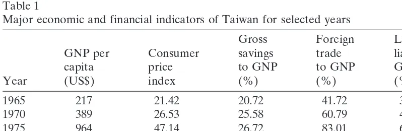
Table 1
Major economic and financial indicators of Taiwan for selected years
Gross Foreign Liquid
GNP per Consumer savings trade liability to Total
capita price to GNP to GNP GDP no. of
Year (US$) index (%) (%) (%) banks
1965 217 21.42 20.72 41.72 34.84 17
1970 389 26.53 25.58 60.79 42.58 21
1975 964 47.14 26.72 83.01 60.08 28
1980 2344 71.45 32.28 106.41 69.81 37
1985 3297 86.58 33.57 93.08 115.13 49
1990 8111 96.51 29.15 87.75 162.74 58
1995 12396 115.98 25.34 94.57 204.88 80
Sources:National Income of Taiwan Area, the ROC(Taipei: Directorate-General of Budget, Account-ing, and Statistics, various issues), Statistical Yearbook of the ROC (Taipei: Directorate-General of Budget),Accounting and Statistics(various issues),Quarterly National Economic Trends, Taiwan Area, the ROC(Taipei: Directorate-General of Budget, Accounting, and Statistics, various issues),Financial Statistics(Taipei: Central Bank of China, various issues).
Base year 1991 as 100.
3.1. A brief review on the financial development in Taiwan
Although Taiwan is a resources-poor small island, its development experience has usually been regarded as spectacular. In addition to the magnificent growth of output and foreign trade, price stability and income distribution equality over the past decades
make Taiwan one of the ‘economic miracles’ of East Asia.10 The first four columns
of Table 1 give a brief view of the per capita GNP, the consumer price index, the ratio of national savings to GNP, and the ratio of export-cum-import to GNP in Taiwan, for selected years.
Development of the financial system in Taiwan definitely contributed to the island’s success by means of stimulating and mobilizing savings as well as allocating investment funds. The last two columns of Table 1 list the ratio of liquid liability to GDP and the number of commercial banks (both domestic and foreign) in Taiwan, which give a rough measure of the level of financial development. It is shown that the financial system grew steadily over the sample period. Nevertheless, the system has often been considered to be sluggish and inefficient. It was even reckoned, in the 1980s, as an obstacle to further economic growth. As in many other LDCs, one of the most significant features of the financial system in Taiwan is the ‘financial dualism,’ which means that, in addition to the formal or organized system, there is also an informal or unorganized system playing a crucial role in financial intermediation. While the formal system consists of banks and monetary institutions which are supervised by the Ministry of Finance and/or the Central Bank of China, the informal system includes those markets and mechanisms where lending and borrowing activities take place without the direct supervision of the financial authorities.11
and competitive. The presumed benefits of financial repression could be undermined at the same time the pressures to develop a more market-based formal financial system intensify. The government has recognized that the backwardness of the financial system would hold back the pace of economic growth and since the late 1970s has administered several measures to reduce the interference and regulations. Liberaliza-tion and internaLiberaliza-tionalizaLiberaliza-tion are the leading principles of financial reform. As far as liberalization is concerned, much effort has been devoted to the areas of interest rate decontrol, market entry deregulation, and privatization of commercial banks. Until now the most successful endeavor has been realized in the matter of interest rates. Six major steps were adopted between 1976—when a formal money market was established—and 1989, when interest controls were totally removed. Fifteen new domestic banks were allowed to commence operations at the end of 1991, a year that marked the elimination of entry barriers. However, the efforts to privatize commercial banks has not paid off as much as anticipated due to strong opposition from vested interest groups.
In addition, the stock market was reformed towards competition in the course of liberalization and the insurance business was forced to open markets to foreign
compa-nies in response to pressure from the United States in the late 1980s.12 In summary,
it is indeed difficult to search for a balance among prudence, stability, and efficiency in macroeconomic management, and Taiwan has traded a lot of efficiency for stability in the course of development. Now Taiwan has to improve its efficiency in financial operations to meet the challenge of economic growth in the future.
3.2. Data description
In empirical application of the two-sector model to the case of Taiwan, we confine our study to examining the relationship between the financial sector and the industrial sector. The financial sector defined in the article consists of four subsectors in the tertiary industry, namely, money and banking, securities and futures, insurance, and real estate brokerage. The industrial sector contains all the subsectors in the secondary industry (i.e., mining and quarrying, manufacturing, utilities, and construction).13
All variables are annual observations from 1961 to 1996. Output in each sector is
measured in terms of value added. The aggregate real output (Yt) is simply the sum
of outputs of both sectors. Capital inputs are defined as the net capital stocks being adjusted by the utilization rates.14Both the capital and output variables are deflated
and expressed in constant prices as of the year 1991. A detailed description of the data sources is given in the Appendix.
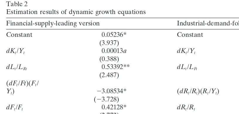
3.3. Estimation results
Upon imposing cross-equation restrictions, regression Eqs. (18) and (19) are esti-mated by using the Seemingly Unrelated Regression Estimation (SURE) method, a
special technique of simultaneous equations system.15 Results are reported in Table
Table 2
Estimation results of dynamic growth equations
Financial-supply-leading version Industrial-demand-following version
System weighted MSE: 1.0199 with 59 degrees of freedom System weighted R2: 0.9226
D-W 1.735 D-W 1.822
Estimated by SURE method with cross equation restrictions: coefficienta in both versions being equal and coefficientbin both versions being equal.
t-values are in parentheses.
* indicates significance level of 1%; ** indicates significance level of 5%; *** indicates significance level of 10%.
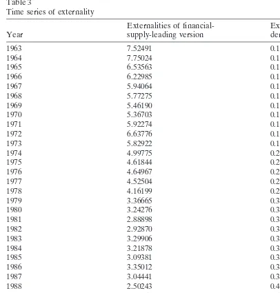
Given the estimated parameters, the marginal externality of each period can be calculated by using the formulas]Rt/]Ft* 5 v(Rt/F*t) and ]Ft/]R*t 5 h(Ft/R*t). They
are tabulated in Table 3. The estimated mean value of the marginal externality of the financial-supply-leading version is 4.02057, while that of the real-demand-following version is 0.33153. It means that the ‘spillover contribution’ of the financial growth onto the industrial growth was greater than that of the reverse case. This outcome seems to imply that the financial-supply-leading profile prevailed in the economy of Taiwan after controlling the factor of productivity differentials between the two sectors. An active expansion of the financial system induces the industrial production to grow and, in turn, increases the demand for its services. Lessening the degree of financial depression and reducing the level of restriction on the financial system are inferred to have positive repercussions on industrialization. This finding seems to conform to the argument advocated by World Bank (1989) and to comply with most of the LDCs surveyed, for example, in Jung (1986). An interesting phenomenon worth mentioning is that the size of the marginal externality of the financial-supply-leading version decreases considerably along with time while that of the real-demand-following version increases. It appears to corroborate Patrick’s (1966) reasoning that the causation changes in the course of development. It runs from the financial side to the real side in the early stage of development, and “as the process of real growth occurs, the supply-leading impetus gradually becomes less important, and the demand-following
Table 3
Time series of externality
Externalities of financial- Externalities of
real-Year supply-leading version demand-following version
4. Time series analysis of the externalities
breaks.17Many econometric techniques have been developed for these purposes. One
of the most commonly used techniques is a regression model incorporating a spline function in time variable. A spline function is a continuous piecewise device whose
pieces are polynomial segments of degree n. The joint points are called knots. A
linear spline (polynomial of degree 1) which is, in general, sensitive to all of the data allows both the intercept and the slope to change between two periods divided by the knot point, but subject to the condition that continuity in time dimension is maintained.18
Assume that there are two knot points occurring at timesaandb.The model used
to detect the structural breaks in an economic time series can be specified as follows:
yt5c01 c1x1t1d1z1t1d2z2t 1d3z3t1 et (20)
where
ytindicates the externality time series,
x1is the vector of economic and financial indicators, and
zjtare the spline time variables with z1t5t; z2t50, as t,a and z2t5t2a, ast >a; and z3t5 0, ast ,band z3t5t2 b, as t>b.
Coefficientd1indicates the time slope before time point a. d2and d3indicates the
change in time slope from beforea to between a and b as well as from between a
and b to after b, respectively. The disturbance term et is assumed to follow the
assumptions of a classical normal linear regression model.19
intensity, which is defined as the net fixed capital stock used per labor, also plays a crucial role in determining the strength of industrial production in the process of industrialization.20
In this study, 1981 and 1989 are chosen as the knot points in the regression Eq. (20). These two years are critical in the recent development process in Taiwan, not only from the perspective of financial liberalization but also from the perspective of industrialization. In 1981 the interest rate deregulation effectively began, and in 1989
the era of financial repression actually ended.21 Upon completion of the Ten Major
Construction Projects, the first large infrastructure construction package in the island, and upon the successful establishment of semi-conductor and other high-technology industries, 1981 was also marked by Li (1988) as the beginning of a new era of ‘the science and technology-oriented.’ 1989 was also the year with significant structural change in aggregate production. In addition to the fact that the share of services outreached the sum of shares of both agriculture and industry, the share of industry actually started to decline.
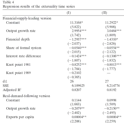
To consider the existence of autocorrelation, the Generalized Least Squares (GLS) method is used in testing the time series of externality. The results of the financial-supply-leading version are presented in the upper half of Table 4 and those of the real-demand-following version are in the lower half.22It is seen that the
goodness-of-fit statistics of all variants are highly satisfactory and most of the explanatory variables are significant. At first, the output growth rate is a significant and robust regressor for explaining the spillover series of both versions. It reveals a positive relation with the supply-leading externalities but a negative one with the demand-following external-ities. Second, the financial depth, the share of the formal system, and the interest rate difference are robust in explaining the variations in the externality of the financial-supply-leading version. They all generate significant negative marginal effects on the series, holding other variables unchanged. Third, although the coefficient estimate of the knot point 1981 is significantly different (at 10% level) from zero in the supply-leading version, that of the knot point 1989 is not significant at all. Fourth, turning to the results of the real-demand-following version, the export variable is more robust in explaining the variations in the externality series than the capital intensity indicator. Finally, the knot point 1989, rather than 1981, is significant as a structural change point in the demand-following case. In summary, since the generating processes of the externality are made by distinct groups of agents in distinct environment, they reveal divergent patterns not only in the long-term trend but also in the short-term variations. Therefore, different sets of economic variables associated with the different knot-points are effective in explaining the variations in these series.
5. Conclusion
Table 4
Regression results of the externality time series
(I) (II) (III)
Financial-supply-leading version
Constant 11.3168* 11.2922* 11.4257*
(5.822) (5.906) (5.753)
Output growth rate 2.9954*** 3.0464*** 3.4298***
(1.742) (1.809) (1.949)
Financial depth 21.2937*** 21.4310* 21.9875*
(22.037) (22.826) (24.897)
Share of formal system 20.0540*** 20.0554** 20.0505***
(22.015) (22.122) (21.879)
Interest rate difference 20.1424*** (20.1306*** 20.1522**
(21.807) (21.832) (22.074)
Knot point 1981 20.8252*** 20.8013*** —
(21.784) (21.777)
Knot point 1989 20.2102 — —
(20.365)
d.f. 26 27 28
SSE 6.109625 6.214774 7.055775
Adjusted R2 0.8207 0.8192 0.8045
Real-demand-following version
Constant 0.1144 0.0998 0.0692
(1.663) (1.509) (0.894)
Output growth rate 20.2079** 20.2150** 20.2341**
(22.402) (22.495) (22.230)
Exports per capita 0.00004** 0.00004** 0.00006**
(2.208) (2.259) (2.610)
Capital intensity 0.00021 0.00025*** 0.00030***
(1.350) (1.697) (1.741)
Knot point 1981 0.0209 — —
(0.825)
Knot point 1989 0.1080* 0.1023* —
(3.747) (3.656)
d.f. 27 28 29
SSE 0.018117 0.018631 0.027560
Adjusted R2 0.9366 0.9367 0.9215
Estimated by the GLS method. More specifically, a two-step full transform Yule-Walker method in SAS 6.0 package is used.
t-values are in parentheses.
* indicates significance level 1%; ** indicates signifciance level of 5%; *** indicates significance level of 10%.
process. The causation can then be evaluated in terms of the intersectoral externalities estimated from the model. The framework so designed is proposed as an alternative to the Granger causality test, which uses only the statistical techniques without theoretical reasoning.
of the financial-supply-leading version is greater than that of the real-demand-following version. The size of the former declines along with time while that of the latter increases. These findings are compatible with Patrick’s (1966) hypothesis that the supply-leading force dominates at the early stage of development in most LDCs and the causation changes in the course of development. The results also indicate that the variations in externality series of the financial sector of the supply-leading version can be explained mostly by the financial variables, such as the financial depth, the share of formal finance, and the interest difference. The variations in externality series of the industrial sector of the demand-following version can be explained by the real economic variables, which largely determine the industrial production.
The findings in the present study suggest that there exists much room for future research in this area. Since the unorganized financial market usually plays a substantial role in LDCs, its functions and effects on the real sector and on the entire economy will definitely be consequential. Excluding it from the study might cause the results to be biased. Emphasizing the role of an informal sector might shed some light on the exact nature of financial development.
Acknowledgments
The author is grateful to Professors W.J. Hsieh, Y.H. Yang, Y.L. Wang, and F.S. Hung and, in particular, to anonymous reviewers for their constructive comments and suggestions. All remaining errors are the author’s.
Appendix
Sources of data
National Income of Taiwan Area, ROC, various issues
Outputs of real sector and financial sectors GDP deflator
GDP in market value at current prices Capital formation price index
The Trends in Multifactor Productivity, Taiwan Area, ROC, various issues
Net fixed capital stock in constant prices 1991 Net fixed capital intensity (per labor unit)
Monthly Statistics of Industrial Productivity, various issues
Capital utilization rate
Quarterly National Income Statistics in Taiwan Area, ROC(1996)
Liquid Liability
Taiwan Statistical Data Book, various issues.
Shea and Yang (1997), modified by author Share of formal financial system Shea (1994), modified by author
Interest rate difference
Notes
1. See, for example, World Bank (1989) for illustration.
2. A macroeconomic environment with strategic complementarity is an environ-ment in which the incentive for agent to produce is larger the higher the aggregate production. Cooper and John (1988) provide a useful discussion of strategic complemnetarity and its role in generating equilibrium in model economies.
3. For insightful discussions, see Greenwood and Jovanovic (1990) and Bencivenga and Smith (1991).
4. This formulation is motivated by the Lucas’ aggregate supply story that specifies expectation errors about prices as a source of variations in output. See Lucas (1973) for details.
5. One of the essential merits of adaptive expectations over other more compli-cated theses, such as that of rational expectations, is that it can readily be incorporated into econometric modeling exercises and be subject to empirical testing.
6. It is noticed that the focal point of this study is on the spillover externality gauged in terms of physical production. In the literature of two-sector model with emphasis on production externality between sectors (e.g., Feder, 1983; Odedokun, 1996), the role of relative prices was not specified explicitly. Any relative price ratio introduced in model specification will eventually be lost to sight in the process of deriving the estimatible growth equations that follow. 7. The definition and properties of a neoclassical well-behaved production function
are particularly appropriate and useful in studying production behavior at the industry or firm level. For further discussion, see Chamber (1988), Chapter 1. 8. In empirical study, these constraints could be relaxed if the two sectors in
question do not make up the entire economy.
9. This is shown in most of the econometric textbooks involving time series models (e.g., Pindyck & Rubinfeld, 1991, pp. 206–208).
10. Even since the summer of 1997 when the financial crisis broke up in Asia, Taiwan’s economic performance has remained better than that of other coun-tries of the region.
12. For a more detailed and informative discussion regarding Taiwan’s financial reform see Shea (1994); Yang (1994); and Shea and Yang (1997).
13. The entire agricultural sector and most subsectors in the tertiary industry (except the financial sector) are not included in the study mainly because no reliable capital data of these sectors are available. The empirical study so performed is considered as a partial equilibrium analysis. It is believed that the exclusion will not affect the implications of the model.
14. The capital utilization rate of the manufacturing sector is used as a proxy throughout the study since there is no such indicator compiled for other sectors. 15. See, for example, Greene (1993), Chapter 17 for details.
16. Patrick (1966, p. 177).
17. In case studies regarding Korea, Indonesia, and Malaysia, Kitagawa (1995) examined the structural changes brought on by financial liberalization in these countries using the Chow test method.
18. Setting the function to be continuous at the knot points is a major advantage of the spline function model over other techniques on checking structural changes. For further discussion of the model and its applications, see Poirier (1973), and Poirier and Garber (1974).
19. These assumptions are subject to testing in empirical applications. See Poirier and Garber (1974) for discussion.
20. The data sources of these explanatory variables are also listed in the Appendix. 21. See Shea (1994) and Shea and Yang (1997).
22. The time trend tis omitted to avoid the problem of multicollinearity among
regressors.
References
Arestis, P., & Demetriades, P. (1997). Financial development and economic growth: Assessing the evidence.The Economic Journal 107(May), 783–799.
Bencivenga, V. R., & Smith, B. D. (1991). Financial intermediation and endogenous growth.The Review of Economic Studies 58, 195–209.
Chamber, R. G. (1988).Applied Production Analysis: A Dual Approach.Cambridge: Cambridge Univer-sity Press.
Cooper, R., & John, A. (1988). Coordinating coordination failures in Keynesian models.Quarterly Journal of Economics 103(3), 441–463.
De Gregorio, J., & Guidotti, P. E. (1995). Financial development and economic growth.World Develop-ment 23(3), 433–448.
Demetriades, P. O., & Hussein, K. A. (1996). Does financial development cause economic growth? Time-series evidence from 16 countries.Journal of Development Economics 51, 387–411.
Feder, G. (1983). On exports and economic growth.Journal of Development Economics 12, 59–73. Fritz, R. G. (1984). Time series evidence on the causal relationship between financial deepening and
economic development.Journal of Economic Development 9, 91–111.
Fry, M. J. (1982). Models of financial repressed developing economies.World Development 10(9), 731–750. Fry, M. J. (1997). In favour of financial liberalisation.The Economic Journal 107(May), 754–770. Galbis, V. (1977). Financial intermediation and economic growth in less developed countries: a theoretical
Goldsmith, R. W. (1969).Financial Structure and Development.New Haven: Yale University Press. Greene, W. H. (1993).Econometric Analysis(2nded.). New York: Macmillan.
Greenwood, J., & Jovanovic, B. (1990). Financial development, growth and the distribution of income.
Journal of Political Economy 98, 1076–1107.
Jung, W. S. (1986). Financial development and economic growth: international evidence. Economic Development and Cultural Change 35, 333–346.
King, R. G., & Levine, R. (1993). Finance and growth: Schumpeter might be ‘right’.Quarterly Journal of Economics 108, 717–737.
Kitagawa, H. (1995). Financial liberalization in Asian countries. In T. Kawagoe & S. Sekiguchi (Eds.),
East Asian Economies: Transformation and Challenges(pp. 139–171). Singapore: Institute of Southeast Asian Studies.
Li, K. T. (1988). The Evolution of Policy behind Taiwan’s Development Success. New Haven: Yale University Press.
Lucas, R. E. (1973). Some international evidence on output-inflation tradeoffs. American Economic Review 63, 326–334.
Mathieson, D. J. (1980). Financial reform and stabilization policy in a developing economy.Journal of Development Economics 7(3), 359–395.
McKinnon, R. I. (1973).Money and Capital in Economic Development.Washington, D.C.: The Brookings Institution.
Murinde, V., & Eng, F. S. H. (1994). Financial development and economic growth in Singapore: demand-following or supply-leading?Applied Financial Economics 4, 391–404.
Nerlove, M. (1958). Adaptive expectations and cobweb phenomena.Quarterly Journal of Economics 73, 227–240.
Odedokun, M. O. (1996). Alternative econometric approaches for analyzing the role of the financial sector in economic growth: time-series evidence from LDCs.Journal of Development Economics 50, 119–146.
Pagano, M. (1993). Financial markets and growth: an overview.European Economic Review 37, 613–622. Patrick, H. T. (1966). Financial development and economic growth in under-developed countries.
Eco-nomic Development and Cultural Change 14, 174–189.
Pindyck, R. S., & Rubinfeld, D. (1991).Econometric Models and Economic Forecasts(3rd ed.). New York: McGraw-Hill.
Poirier, D. J. (1973). Piecewise regression using cubic spline.Journal of the American Statistical Association 68, 515–524.
Poirier D. J., & Garber, S. G. (1974). The determinants of aerospace profit rates 1951–1971.Southern Economic Journal 41, 228–238.
Quarterly National Income Statistics in Taiwan Area, ROC.(1996). Taipei: Directorate-General of Budget, Accounting and Statistics.
Ram, R. (1987). Exports and economic growth in developing countries: evidence from time-series and cross-section data.Economic Development and Cultural Change 36(1), 51–72.
Roubini, N., & Sala-i-Martin, X. (1992). Financial repression and economic growth.Journal of Develop-ment Economics 39(July), 5–30.
Shaw, E. S. (1973).Financial Deepening in Economic Development.New York: Oxford University Press. Shea, J. D. (1994). Taiwan: development and structural change of the financial system. In H. T. Patrick & Y. C. Park (Eds.),The Financial Development of Japan, Korea, and Taiwan: Growth, Repression, and Liberalization(pp. 222–287). New York: Oxford University Press.
Shea, J. D., & Yang Y. H. (1997). Financial system and economic development in Taiwan. In T. S. Yu & J. S. Lee (Eds.),Economic Policies and Economic Development(pp. 149–190). Taipei: Chung-Hua Institute for Economic Research. (In Chinese).
Spears, A. (1991). Financial development and economic growth-causality tests.Atlantic Economic Journal 19(3), 66.
Wang, E. C. (1999). Externalities between financial and real sectors in the development process. Interna-tional Advances in Economic Research 5(1), 149–150.
World Bank (1989).World Development Report 1989: Financial Systems and Development.New York: Oxford University Press.