The in
#
uence of shop characteristics on workload control
Bas Oosterman, Martin Land*, Gerard Gaalman
Faculty of Management and Organisation, University of Groningen, P.O. Box 800, 9700 AV Groningen, Netherlands
Received 9 October 1998; accepted 20 December 1999
Abstract
Several order release methods have been developed for workload control in job shop production. The release methods of the traditional workload control concepts di!er in how they deal with the#ow of work to each station. Previous research has pointed at strengths and weaknesses of each method. Till now the choice of the appropriate method for a particular situation has hardly received attention. This research shows that shop characteristics are an important factor to this choice. A simulation study indicates that the relative performance of the release methods changes completely with for instance the presence or absence of a dominant#ow direction in the shop. Adjustments to the traditional release methods are suggested which prove to make these methods more robust. ( 2000 Elsevier Science B.V. All rights reserved.
Keywords: Job shop; Flow shop; Workload control; Order release
1. Introduction
An important category of production control approaches for job shop production is based on workload control (WLC) principles. The WLC con-cepts bu!er the shop#oor against the dynamics of arriving orders by means of input/output control. The order release decision is the main instrument for the input control. Once released, a job remains on the shop#oor until all its operations have been completed. WLC concepts set norms for the work-load allowed on the #oor. If a job does not "t in these norms, the release decision will hold it back. This results in a pool of unreleased jobs.
*Corresponding author. Tel.: #31-503637188; Fax #31-503632032.
E-mail address:[email protected] (M. Land).
WLC has received a lot of attention from both practitioners and researchers. Practitioners appreciate the concepts, because they correspond with their intuitive ways of controlling shops. Moreover, they expect practical support in taking decisions. Researchers developed several concepts and workload controlling release methods. Pure job shop models have been used for evaluation, as the concepts were mainly developed for job shop environments. Few researchers have stressed the importance to test the concepts in more realistic situations that deviate from the pure job shop [1,2]. In a pure job shop model the#ows of jobs are undirected, routing sequences are completely ran-dom. However, in most real life shops we generally distinguish a dominant#ow direction, with work-stations having di!erent positions in this#ow. As each of the WLC concepts deals di!erently with the
#ow of work to these stations, one may expect these
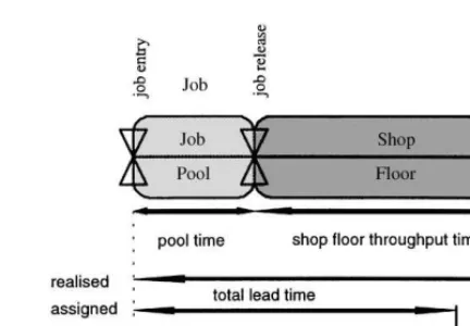
Fig. 1. Lead time components with controlled release.
deviating characteristics to have in#uence on the performance of WLC concepts. In this paper we analyse this in#uence. By means of a simulation study, di!erent shop con"gurations are examined. The tested WLC concepts are three traditional con-cepts and two recently developed alternatives [3]. Preliminary simulation results have been discussed in [4].
The results of this study should contribute to the choice of an appropriate workload control in a practical situation. As there still is a lot of con-fusion on the gap between theoretical and practical results of WLC concepts, the simulation of more realistic shops may also contribute to our under-standing of this gap.
The paper is organised as follows. First, we describe the basic principles of workload control and give a detailed analysis of di!erences between the release methods of WLC concepts. Next, we formulate our expectations with respect to the in#uence of shop characteristics on each of these methods. Section 5 discusses the experimental design of the simulation study to verify these expec-tations. Sections 6 and 7 deal with the results and the implications of the study.
2. The workload control (WLC) concept and job release
An important decision within WLC concepts is job release (see [5,6] for thorough reviews of job release research. Job release determines when each job should enter the shop #oor. Once released, a job remains on the #oor until all its operations have been completed. The progress of jobs on the shop#oor is controlled by priority dispatching in the queues at work stations. The principle of WLC concepts is to control these queues. Norms are set for the workload allowed on the shop#oor. If a job does not"t in these norms, the release decision will hold it back. It results in apoolof unreleased jobs. This pool may absorb#uctuations of the incoming
#ow of orders. Besides a reduction of work-in-process costs, holding back jobs has numerous additional advantages. It creates a transparent shop #oor situation with faster feedback oppor-tunities, which is of great importance in the
turbulent job shop situation. JIT literature exten-sively presents the bene"ts of a lean shop#oor. In addition to these bene"ts, the time jobs spend in the pool enables the delay of decisions. It reduces the waste due to cancelled orders, facilitates later ordering of raw materials, takes away the need of expediting rush orders on the shop #oor, etc. As illustrated by Fig. 1, we refer to the waiting time in the pool as thepool timeof a job and to the time that passes between release and completion of the job as itsshopyoor throughput timeor shortlyshop yoor time. The shop #oor throughput time of the job can be subdivided intostation throughput times. Control of the queues on the shop #oor should result in stable and predictable station throughput times. Thus, an accurate release moment for each job can be determined to guarantee a good due date performance. However, it can be argued that a good timing of job release may con#ict with realising the norms for the workload on the shop
#oor [7].
3. Three approaches of workload control
The workload released for a station can be sub-divided into adirectpart (work from jobs queuing at the considered station) and an indirect or
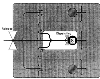
Fig. 2. Inputs to the direct load of a workstations.
cannot completely control the direct load of a work station. Only a part of the jobs in the pool are released directly to the work station. Other jobs arrive from the other work stations after their up-stream operationshave been completed.
Fig. 2 shows the#ows on the shop#oor of a job shop. The simpli"ed context of three stations illus-trates how job release in#uences part of the inputs of workstation sdirectly (1), while other inputs to the direct load ofsarrive from other workstations (2). Di!erent approaches have been proposed, which all aim at keeping the direct load at a low and stable level.
(A) The WLC concept developed at the IFA in Hannover [8}11] estimates the input from jobs upstream to the direct load of a station. The estimated direct loads are subjected to norms.
(B) The WLC concepts developed in Eindhoven [12] and Lancaster [13}15] avoid estimating the input to the direct loads. They aggregate the direct and the indirect workload of a sta-tion by simply adding them and subject this
aggregate workloadto a norm.
(C) Some implementations of the Lancaster con-cept use an alternative approach [13] that ex-tends the aggregate workload to what we will
de"ne as theshop load. The shop load of a
sta-tion addista-tionally includes work already com-pleted at the station, but still downstream on
the shop#oor. The shop load of each station is subjected to a norm. This approach has been developed to restrict the required feedback from the shop#oor to completed jobs, instead of completed operations.
All approaches make the release decision period-ically, and focus control on the remaining work-load at the end of the imminent release period. The remaining workload of a station at the end of the release period together with the output during this period is subjected to a norm value. At the begin-ning of the period, a set of jobs is released such that the workload situation at the end of the release period will satisfy the norms. Balance equations may further clarify the di!erence between the three approaches.
Eq. (1) gives the direct load balance of a stations.
DEs#O
s"DBs#Is, (1)
whereDEs the remaining direct load of a stationsat the end of a release period,O
sthe output of station s during the release period, DBs the direct load of stationsat the beginning of the release period and
I
s the input to the directload from jobs arriving
during the release period.
In Eq. (1)DBs is known at the moment of release. The station outputO
s depends on the capacity of sand its utilisation during the release period. The inputI
s comes from jobs already upstream at the
moment of release and from jobs newly released. Since both O
s and Is encompass uncertainties, DEs cannot be determined exactly at the moment of release.
The aggregate load satis"es balance equation (2).
(DEs#;E
s)#Os"(DBs#;Bs)#Rs, (2)
where;E
s the load upstream of stationsat the end
of the release period, ;B
s the load upstream of
station s at the beginning of the release period,
R
s the input to the aggregate load from newly
released jobs and the other variables are de"ned as before.
The shop load satis"es Eq. (3):
(DEs#;E
s#<Es)#Zs"(DsB#;Bs#<Bs)#Rs, (3)
where <E
s is the load completed by station s, but
still downstream at the end of the release period,
<B
s the load completed by stations, but still
down-stream at the beginning of the release period and
Z
s the output of station s which leaves the shop #oor during the release period.
As in Eq. (2), all the right-hand-side quantities of Eq. (3) are completely known upon the moment of release, and thus the sum of the left-hand quantities can be determined exactly.
Notice that Eq. (1) di!ers from Eqs. (2) and (3) regarding the input, and that Eq. (3) di!ers from Eqs. (1) and (2) regarding the output. In the system of Eq. (1) a job is part of the input as it arrives at the queue of stations, where in Eqs. (2) and (3) the job becomes part of the input directly upon its release. In the systems of both Eqs. (1) and (2) the jobs become part of the considered output as soon as they leave the station, in Eq. (3) a job does not become part of the output until it has left the#oor. Approaches A}C can be related to, respectively, Eqs. (1)}(3).
Approach A controls the direct loadDEs by bring-ing an estimation of the right-hand side of Eq. (1) to a norm level. The input is roughly estimated by a method calledload conversion[9,11]. As soon as a job is released, its processing time partly contributes to the input estimation, the contribu-tion increases as the job progresses on its routing upstream. The whole of the direct load and the estimated input is indicated as the converted load. The norm for the converted load should be set at the desired level (NDs) for the direct loadDEs plus an allowance (N0s) for the estimated output during the release period.
Approach B focuses on the aggregate load (DEs#;E
s). The right-hand side of Eq. (2), which
does not require any estimation, is brought to a norm level. In this case, the norm value should be set at the desired level (NAs) for the aggregate load (DEs#;E
s) plus an allowance (N0s) for the estimated
output during the release period. The aggregate load at the end of the release period (DEs#;E
s) can
be determined upon release, except for#uctuations in the station outputO
s.
Approach C is comparable to B. Here, a norm (NFs) is speci"ed for the shop load (DEs#;E
s#<Es).
The output of sleaving the shop #oor is treated analogously to the direct output of the station. Note that a job contributes to the shop loads of all stations in its routing until it leaves the shop#oor. Upon the completion of a full job, its operation processing times are removed from the shop load records for all stations in its routing. This avoids the need to record the completion of each opera-tion.
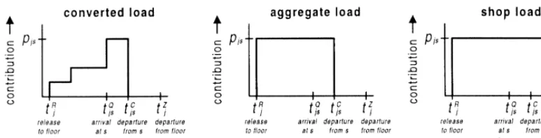
In the above equations we distinguished the direct load, the aggregate load and the shop load of a station. Each load can be de"ned as the joint operation processing times of a certain set of jobs. Each of the balance equations relates to a di!erent set of jobs. Alternatively, we can illustrate the di!erence between the three workload control approaches by following a single job on its routing. Consider a jobjwith an operation processing time
p
js on stations. Say that the job is released at time tRj, enters the queue of stationsattQjs, is completed at stationsattCjsand leaves the#oor attZj. Then, the operation processing time of the job will be part of the direct load during the interval [tQjs,tCjs], it will be part of the aggregate load during the interval [tRj,
tCjs] and part of the shop load during [tRj, tZj]. Fig. 3 depicts the contribution of the job to, respec-tively, the converted load, the aggregate load and the shop load of station s in the course of time. Note that the converted load of approach A includes an estimation of the direct load input, in addition to the direct load itself. Upon release, the job starts contributing to the input estimation. Fig. 3 shows how the contribution increases after each completed operation upstream.
Fig. 3. The contribution of jobjacross time to the workload (methods A}C).
s(tQjs). The direct load is fully included in the con-verted load. Between release and arrival at station
sthe processing time of jobjis partly included in the converted load, as an element of the estimated input.
4. Expected in6uences of shop characteristics
This research started from the perspective that pure job shops do not exist. In every real life job shop there will be more or less dominant #ow direction. The operations performed by some sta-tions have a preparative character (gateways or upstream stations), other stations perform typical
"nishing operations (downstream or "nishing
sta-tions). Finishing stations will have most of their load upstream, while typical gateways have a lot of completed work downstream on the #oor. As we observed that the three workload control approaches di!er with respect to inclusion of upstream and downstream workload, we do expect that the #ow characteristics will have a di!erent in#uence on each of the approaches.
Method A tries to determine the in#uence of release on the direct loads of all stations. In the theoretical pure job shop this is well possible, because part of the jobs reaches the station rather directly after release. But in shops with a more directed#ow, the release of new work in#uences the direct load of a downstream station only after a time lag. Here, we question the usefulness of focussing on the direct load.
Also a second point indicates that method A is particularly developed for the strong routing var-iety of a pure job shop. The estimation of inputs
uses information on the distance of the jobs upstream to the station. As routings vary strongly this information is important to enable a smooth
#ow of jobs to each station. When routing variety is small, this information loses its weight, as we al-ready use workload norms for each station. The fact that also the more upstream stations reach their norm level might ensure a smooth in#ow of work for downstream stations, so input estimation becomes less advantageous.
In method B work upstream of a station is included in its aggregate workload, and the aggregate workloads are subjected to workload norms. For a typical downstream station, it seems reasonable to keep this aggregate workload on a constant level. Its direct load will follow. For a pure job shop, the implications of a constant aggregate load for the direct load are less trivial.
More particularly, the position of a station in the routings of the job is an important factor. When the position of a station is more downstream in the
#ow of the jobs, there will be more load upstream of this station. In a pure job shop the position of each station varies strongly within the mix of routings, which may not allow for the use of"xed norm levels for the aggregate load. Previous research [16] already indicates that method B performs worse than method A in a pure job shop. It is interesting
to "nd out whether the relative performance
of method B improves when the position of each station in the mix of routings is quite stable, which is the case with more#ow shop like routing characteristics.
However, the information whether jobs have passed a speci"c station gets lost with this inclu-sion, while jobs that passed a station are no longer of interest for control of its direct load. Especially for a typical gateway station this loss of informa-tion may be undesirable. So in shops with a domi-nant #ow direction we expect that the detailed recording of completed operations in method B gives an important advantage over method C.
A more speci"c consideration with respect to method C relates to the number of operations per job. The direct load of a station, which should be controlled, may be only a small part of the shop load. The share of the direct load depends on the number of other operations that have to be per-formed on each job. The higher the number of operations, the larger the shop load should be to get the same share of the direct load. The number of operations per job generally varies strongly in pure job shops. This may have a negative in#uence on approach C that applies a constant norm level to the shop loads. Previous research of the authors [3] studies an alternative approach that corrects the shop load for the number of operations. This ap-proach completely outperforms apap-proach C in a pure job shop. This raises the question whether the relative performance of approach C improves in shops with a rather constant number of operations.
5. Experimental design
The previous section stated our expectations with respect to the in#uence of the shop con" gura-tion on each of the workload control approaches. We will analyse these in#uences by means of a simulation study. This section details the release methods and the shop con"gurations to be simulated.
5.1. Release methods
In addition to the release methods A}C, two alternative methods are included in the experi-mental design. The previous section suggested some particular in#uences of the station position and the number of operations in respectively method B and C. Previous research of the authors
[3] studies an alternative approach which corrects aggregated loads for the suggested in#uences. Two variants of this approach will be included in the experimental design to verify the expected in#uences, as alternatives for, respectively, methods B and C. The alternatives will be indicated as B@
and C@.
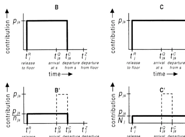
Method B@ uses the same timing of input and output as method B. A job is included in the re-corded load of stationsdirectly upon release, and excluded as soon as the operation at station s is completed. The di!erence between method B and B@ relates to the contribution of the job to the recorded load. Instead of a contribution p
js (the
processing time of a job j at station s), the job contributes p
js/njs (during the same interval [tRj, tCjs]). Heren
js is de"ned as the position of station sin routing of jobj, in other words: stationsis the
n
jsth station that job j will visit. The left part of
Fig. 4 depicts the workload recordings of method B and B@. We suggested that the aggregate load should increase when stationsis more downstream in the momentary#ow of jobs. Note that the work-load calculation of method B@ automatically corrects for this factor. The expected in#uences of the station position can now be veri"ed by perfor-mance di!erences between B and B@.
Method C@ is comparable to method C with respect to the timing of input and output. A job
j contributes to the recorded workload of station
sduring the interval [tRj,tZj]. Here the contribution of jobjis decreased top
js/Nj, whereNj is de"ned
as the number of operations to be performed for job
j, or the routing length. Where the shop load should increase when the momentary mix of jobs has a larger number of operations to be performed, method C@ corrects for this factor. The di!erence between methods C and C@is illustrated in the right part of Fig. 4. Including C@ helps in verifying the expected in#uences of the routing length.
Fig. 4. Methods B@and C@: adjusting job contributions to the workloads.
The estimation is based on the assumption that the station throughput times are equal for all stations in the routing of a job. In that case 1/n
js"(tCjs!tQjs)/(tCjs!tRj) and 1/Nj"(tCjs!tQjs)/
(tZj!tR
j). In Fig. 4 the contribution of a job to the
direct load across time is given by a dashed curve. We can see that, given the above assumption, the average contribution of a job in the workload cal-culation of methods B@ and C@ during an interval including at least [tRj,tZj] will be equal to its average contribution to the direct load during that interval. A norm for the workload calculated in methods B@
and C@can be seen as a norm for the average direct load.
The "ve methods included in the experimental
design di!er with respect to the quantities that are subjected to workload norms. The release proced-ure is implemented equally for all methods. Upon arrival the jobs are sequenced in the pool according to planned released times. This planned release time is determined by subtractingN
jtimes a
stan-dard station throughput time from the due date of the job. Periodically (once a week), the release deci-sion is made. In order of planned release times, the jobs are considered for release. A job is only se-lected for release, if its release does not cause the
workload norm of any station to be exceeded. After selection, the job is included in the workloads. All jobs in the pool are considered, but according to the pool sequence, jobs with an earlier planned release time have a higher probability to be selected. Jobs that are not selected have to wait in the pool until the next release time. The load conversion procedure of method A is implemented as described in [9].
After release to the#oor, the jobs are sequenced
&"rst-come-"rst-served'in the queue of each station.
5.2. Shop conxgurations
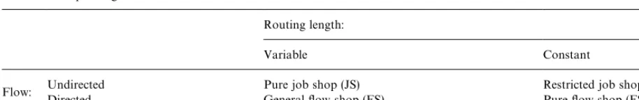
Table 1
Simulated shop con"gurations
Routing length:
Variable Constant
Undirected Pure job shop (JS) Restricted job shop (RJS)
Flow:
Directed General#ow shop (FS) Pure#ow shop (FS)
Enns [1] argues that real life job shops have most in common with the theoreticalgeneralyow shop. In the theoreticalpureyow shop, each job has exactly the same routing. However in a general#ow shop, a movement between any combination of two stations may occur, but the #ow will always have the same direction. Compared to the pure #ow shop routing, any set of stations might be excluded from the routing. Thus, the general#ow shop may still show routing variety with respect to routing lengths, though there is one#ow direction.
Including arestricted job shopwith variable rout-ing sequences and constant routrout-ing lengths com-pletes the spectrum between a pure job shop and a pure #ow shop. This results in a matrix of four shop con"gurations (Table 1). These con"gurations bound the spectrum, within which most real life job shops will fall.
The four shop con"gurations have been
modelled for simulation as follows.
The pure job shop model (JS) of Melnyk et al. [17] has been the starting point of our study. This shop consists of six stations. No station performs more than one operation of a job. This means that return visits do not occur, and that the maximum number of operations per job is limited to 6. More precisely, the lengths of the job routings are deter-mined by drawing from a discrete uniform distribu-tion on [1,6]. The routing sequence is completely random.
The routings in the general#ow shop (GFS) are determined equally, only will the stations be visited in order of increasing station number. Thus, the number of stations to be visited by a job (N
j) is
drawn"rst (from the discrete uniform distribution on [1,6]). Next, a random set of N
j stations is
selected and sequenced in order of increasing sta-tion number. Thus, if stasta-tion 1 is part of the selected
set it will always be the "rst station in the job routing, and if station 6 is selected it will always be last.
In the restricted job shop (RJS) each job visits all stations. But, the sequence of the visits is com-pletely random.
In the pure#ow shop (FS) each job visits all six stations in order of increasing station number.
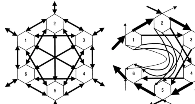
The routing of a job is determined directly upon its arrival in each of the simulated con"gurations. Fig. 5 gives an impression of the resulting#ows in the pure job shop and the general#ow shop. The thickness of the lines indicates the size of the#ows. In all shop con"gurations the average operation processing time is the same (1 day). The job shop
con"guration of Melnyk et al. [17] uses
exponenti-ally distributed processing times. Instead, we use a 2-erlang distribution, which better approaches our observations in real life job shops. The same average utilisation level of 90% is created in each shop by setting the appropriate arrival rate. Jobs arrive according to a Poisson process.
5.3. Workload norms and performance measurement
For each of the release methods, appropriate values for the workload norms have to be deter-mined. In particular, we want to compare the methods at di!erent levels of norm tightness. In each shop con"guration we simulated nine norm levels (including in"nity) for each release method. Since each method uses di!erent workload ag-gregations, it is di$cult to set comparable norm levels. To compare the release methods at di!erent levels of norm tightness, we use the average shop
#oor time as an intermediate variable.
Fig. 5. Flows in (a) the pure job shop; (b) the general#ow shop.
same average shop#oor time. Therefore, the simu-lation results will be presented graphically, with the performance measure set against the shop #oor time. Note that the average shop #oor time of the jobs will decrease when the workload norms for release to the#oor are set tighter.
Norms must be set for each station. For methods A, B@, C and C@ the norms are set equal for all stations. In the cases of directed#ows the aggregate loads in method B requires higher norms the more a station is positioned downstream. In these cases we relate the norm for each station to its recorded aggregate load for in"nite norms.
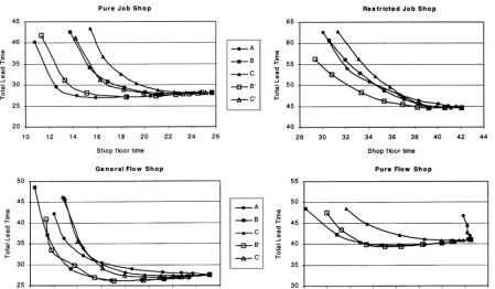
6. Simulation results
Fig. 6 shows the lead time performance for each of the four simulated shop con"gurations. The average total lead time (see Fig. 1) is plotted against the average shop #oor time. For each release method a curve is constructed. A mark on the curves is the result of simulating a release method with a speci"c norm level. As we simulated nine norm levels per method, each curve contains nine marks. A mark is the result of 50 simulation runs of 6000 days, including a start-up period of 2000 days. The common random numbers technique has been used to reduce variance between experiments.
When the curve of one method remains below the curve of another, we may say that the former one shows the better lead time performance. Measures of due date performance have been recorded as well. However, we will not present the exact results here, as the relative due date performance of the simulated release methods did hardly di!er from the presented lead time results. Obviously, due date performance is largely deter-mined by the lead times.
Note that the curves converge at the most right mark. This is the result of the in"nite norm level. As might be expected, all release methods give the same result if release is not restricted by the work-load norms. By lowering the norm levels, the aver-age#oor time decreases. Thus moving from right to left, we see that also the total lead time tends to decrease"rst in most situations. As norms tend to get tighter (to the left end of the curves) total lead times tend to increase. Based on the analogy with semi-open queueing networks [18] several ap-proaches will show asymptotic behaviour at low norms. To which extent the asymptotic behaviour di!ers between release approaches is di$cult to foresee.
Fig. 6. Lead time performance in each of the shop con"guration.
the increasing lead time implies that waiting time in the pool increases stronger than waiting time on the #oor decreases for tighter norms. In the pure job shop we observe that lead times tend increase rather fast as norms get tighter for methods B and C, methods using norms for aggregated workloads. We observe that most simulations presented in job shop literature deal with strongly aggregating workload control methods. Our "ndings might partly explain the negative results reported from these studies. We also see that method A strongly outperforms methods B and C as norms get tighter. Contrary to the other two, method A has quite a large region where the lead time does not in-crease. As was expected, method C shows worse performance than method B. Methods B@ and C@
result in a strong improvement relative to methods B and C.
In the restricted job shop the di!erence between the methods is rather small. All methods result in increasing lead times as norms get tighter. Method B@ outperforms all other methods, including
method A. Method C@gives exactly the same results as method C. Since, the number of stations (N
j) is
6 for each jobj, the relative contribution of each job to the workload will be equal for method C and C@. The general #ow shop sketches a completely di!erent picture. Method B outperforms the others. The correction in method B@ no longer improves method B, and also the di!erence between methods C and C@ is small. Method A shows the worst results at higher shop #oor times. Only at tight norms it improves over method C.
The pure#ow shop shows quite spectacular re-sults. Here method A is not able to reduce the shop
#oor times. As the routing length is the same for all jobs, methods C and C@ give exactly the same re-sults.
7. Discussion of results
The di!erent results found in each of the shop
con"gurations give rise to further analysis. We will
subdivide our discussion into two parts. First, we discuss the in#uence of variable station positions and routing lengths. Next, we assess the in#uence of a directed#ow.
7.1. The inyuence of variable station positions and routing lengths
In the pure job shop method A performs rather well. Methods B and C are not able to realise the same reduction of shop #oor time. In our earlier discussion we suggested that the position of each station varies strongly within the routing mix of a job shop. This might not allow for the use of a constant norm for the aggregate load, as in method B. Since, the aggregate load includes the load upstream of a station, a momentarily in-creased station position will require an inin-creased aggregate load. In the pure job shop, the station position continuously changes within the mix of jobs on the #oor. Our expectation regarding the in#uence of the variable station position is
con-"rmed by the strong improvement that results from
using method B@instead of method B. The station position shows less variation in the job routings of the general #ow shop. In the pure #ow shop the position becomes even invariable. This might ex-plain the strongly improved relative performance of method B in the#ow shop con"gurations.
Regarding method C we expected the variable routing length to con#ict with unchanging shop load norms. As method C@ corrects for routing length di!erences among jobs, the improved perfor-mance of method C@ in the shops with variable routing lengths con"rms our expectations. In the restricted job shop, the performance of method C is closer to that of method B. This also strengthens our argument on the in#uence of the number of operations.
The "xed routing length in the restricted job
shop seems to a!ect all methods negatively, parti-cularly method A. For a possible explanation of this feature, we look at the average position of a station in the job routings. The constant routing length is 6 stations and the average station position is 3.5 in the restricted job shop. In the pure job shop, the average routing length is 3.5 and the average station position in a routing is only 2.25. In the latter case it will be much easier to in#uence the direct load of a station by the release of jobs. As method A estimates the direct in#uence of job release on the direct loads, the di!erence of the average routing length might explain the deterior-ated performance of method A. Further research is needed to explain the in#uence of this factor in more detail.
7.2. The inyuence of a directedyow
Method C is always outperformed by method B. This was expected, because information on com-pleted operations is not used in the shop load of method C. Particularly in shops with a directed
#ow, the shop load of an upstream station hardly gives any information on its direct load situation. The simulation also shows more improvement of method B relative to method C in the #ow shop
con"gurations.
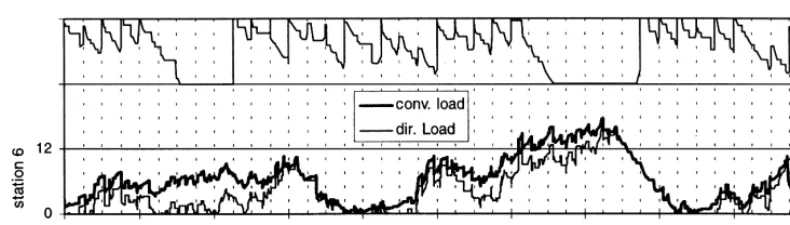
Method A displays curious behaviour in the pure
#ow shop. It becomes completely impossible to reduce the shop#oor time by applying method A. In order to understand this behaviour, we gathered detailed input/output data of the pure #ow shop during one simulation run. Fig. 7 displays the exact course of the direct load for station 1 (the upper part of Fig. 7) and for station 6 (the lower part) during a certain interval. In addition, the value of the converted load is depicted for station 6. Remember that the converted load includes an estimation of the input (from jobs upstream) to the direct load during the next week. As station 1 is the gateway, the converted load of station 1 is exactly equal to its direct load.
Fig. 7. The course of the workloads for method A in a pure#ow shop.
The release of new jobs will not be allowed, if it causes the converted load of any station to exceed the norm level. The workload norms are set tightly at 12 days of work in the presented situation. We see in "gure that at most release times the norm level is exactly reached at station 1. At a certain time, it can be observed that the converted load of station 6 exceeds the norm level. At that time it is not allowed to release any job that contributes to the converted load of station 6. Since, in the pure
#ow shop every job will visit station 6, the release of any job will contribute to the converted load of station 6 (see also Fig. 3). Thus, release is com-pletely blocked. We see that the direct load of station 1 starts to decrease. However, station 6 still receives work from upstream. It takes at least six release periods until the workload of station 6 starts to decrease. In the mean time, we see that station 1 has starved. Since no job has been re-leased for 6 periods, the #ow upstream of station 6 has run dry. As a consequence the direct load of station decreases rather rapidly, and station 6 itself tends to starve. This cyclic pattern explains the disastrous behaviour of method A in a pure #ow shop. Since stations starve too often the utilisation level of 90%, which is required by the arrival rate of the jobs, will not be realised. The pool of jobs waiting for release continues to grow and lead times continue to increase. Thus, the simulation becomes unstable.
This illustrates the danger of reacting on work-load levels of downstream station in situations with more directed#ow. The cyclic behaviour, which we could show explicitly in the pure#ow shop, might occur latently in other shop con"gurations. The
strong performance of method B suggest that it is better to keep aggregate loads (including all work upstream) on a constant level. Perhaps it might be even better to exclude the direct load from the aggregate load and to focus on the quantities upstream in the case of a downstream station. However, verifying this suggestion requires further research.
8. Conclusions
This research started from the perspective that pure job shops do not exist. In every real life job shop there will be a more or less dominant#ow direction. The operations performed by some stations will have a preparative character, other stations will perform typical "nishing operations. Finishing stations have most of their load upstream, while typical gateways have a lot of completed work downstream on the
#oor.
each station. Alternatively, it proved to be useful to adjust the aggregate load of stations (which include work upstream) for variations of the station posi-tion in the job routings or to adjust the shop load (also including work downstream) for the routing length variations. Obviously, the aggregate workload and the shop load do not appropriately indicate the future#ow of work to a station in the case of job shops.
As the #ow becomes increasingly directed, focussing on the direct load might create undesir-able (cyclic) e!ects. In that case aggregate workloads seem to be a more appropriate variable to control. Aggregate workloads do no longer re-quire adjustments.
The"ndings may explain part of the poor
perfor-mance of controlled release methods reported in many simulation studies. These studies often apply release methods that strongly aggregate workloads in a pure job shop model.
This study investigated four shop con"gurations. Reality will be somewhere between these extremes. Knowledge on the performance of each WLC con-cept in these extremes may contribute to the choice of a WLC concept that "ts well to a particular situation. Further research should detail intermedi-ate shop con"gurations and look at robustness with respect to other modelled characteristics such as capacities and processing times. Another impor-tant next step is to detail the analysis of factors that achieve the reductions in total lead times within WLC.
References
[1] S.T. Enns, An integrated system for controlling shop load-ing and work#ows, International Journal of Production Research 33 (10) (1995) 2801}2820.
[2] L.M. Roderick, D.T. Philips, G.L. Hogg, A comparison of order release strategies in production control systems, In-ternational Journal of Production Research 30 (3) (1992) 611}626.
[3] M.J. Land, G.J.C. Gaalman, Towards simple and robust workload norms, Proceedings of Workshop on Produc-tion Planning and Control, Mons, 1996, pp. 66}96.
[4] B. Oosterman, Een vergelijking van werklastbeheersings-methoden in verschillende produktiesituaties. Unpub-lished Master Thesis 1995 (in Dutch).
[5] D. Bergamaschi, R. Cigolini, M. Perona, A. Portioli, Order review and release strategies in a job shop environment: A review and a classi"cation, International Journal of Production Research 35 (2) (1997) 339}420.
[6] H.P.G. van Ooijen, Load-based work-order release and its e!ectiveness on delivery performance improvement, Ph.D. Thesis, University of Eindhoven, The Netherlands, 1996. [7] M.J. Land, G.J.C. Gaalman, Workload control concepts in
job shops: A critical assessment, International Journal of Production Economics 46}47 (1996) 535}548.
[8] W. Bechte, Steuerung der Durchlaufzeit durch belastungs-orientierte Auftragsfreigabe bei Werkstattfertigung. Dissertation VDI-Z Reihe 3, Nr. 70, 1980 (in German). [9] W. Bechte, Theory and practice of load-oriented
manufac-turing control, International Journal of Production Research 26 (3) (1988) 375}395.
[10] W. Bechte, Load-oriented manufacturing control, just-in-time production for job shops, Production Planning and Control 5 (3) (1994) 292}307.
[11] H.-P. Wiendahl, Load-Oriented Manufacturing Control, Springer, Berlin, 1995.
[12] J.W.M. Bertrand, J.C. Wortmann, Production control and information systems for component-manufacturing shops, Dissertation, Elsevier, Amsterdam, The Netherlands, 1981. [13] I.P. Tatsiopoulos, A microcomputer-based interactive sys-tem for managing production and marketing in small component-manufacturing "rms using a hierarchical backlog control and lead time management methodology, Ph.D. Thesis, University of Lancaster, 1983.
[14] L.C. Hendry, A decision support system to manage deliv-ery and manufacturing lead times in make-to-order com-panies, Ph.D. Thesis, University of Lancaster, UK, 1989. [15] B.G. Kingsman, I.P. Tatsiopoulos, L.C. Hendry, A
struc-tural methodology for managing manufacturing lead times in make-to-order companies, European Journal of Opera-tional Research 40 (2) (1989) 196}209.
[16] M.J. Land, G.J.C. Gaalman, The performance of wokload control concepts in job shops: Improving the release method, International Journal of Production Economics 56}57 (1998) 347}364.
[17] S.A. Melnyk, G.L. Ragatz, Order Review/Release Systems: research issues and perspectives, International Journal of Production Research 27 (7) (1989) 1081}1096.
[18] J.A. Buzacott, J.G. Shantikumar, Stochastic Models of Manufacturing Systems, Prentice-Hall, Englewood Cli!s, NJ, 1993.