REACTION-DIFFUSION FRONT SPEEDS IN
SPATIALLY-TEMPORALLY PERIODIC SHEAR FLOWS∗
JIM NOLEN† AND JACK XIN‡
Abstract. We study the asymptotics of two space dimensional reaction-diffusion front speeds through mean zero space-time periodic shears using both analytical and numerical methods. The analysis hinges on traveling fronts and their estimates based on qualitative properties such as mono-tonicity and a priori integral inequalities. The computation uses an explicit second order upwind finite difference method to provide more quantitative information. At small shear amplitudes, front speeds are enhanced by an amount proportional to shear amplitude squared. The proportionality constant has a closed form expression. It decreases with increasing shear temporal frequency and is independent of the form of the known reaction nonlinearities. At large shear amplitudes and for all reaction nonlinearities, the enhanced speeds grow proportional to shear amplitude and are again decreasing with increasing shear temporal frequencies. The results extend previous ones in the liter-ature on front speeds through spatially periodic shears and show front speed slowdown due to shear direction switching in time.
Key words. fronts, space-time periodic shears, speed enhancement, asymptotics, computation
AMS subject classifications. 35K57, 41A60, 65D30
DOI.10.1137/S1540345902420234
1. Introduction. Front propagation in heterogeneous media appears in many scientific disciplines such as combustion of premixed flames, reactive pollutant trans-port in porous media, and invasion of biological species, just to name a few [7], [33], [24], [30]. Though heterogeneities are dominantly spatial in the latter two areas of ap-plication, in combustion, especially turbulent premixed flame problems, a wide range of spatial and temporal scales can arise in the multiscale environment (i.e., fluid ad-vection) where flames are moving; see, e.g., [13], [19], [20], and the references therein. The large time propagation speed of a flame front is an upscaled quantity depending on both flow and chemistry, and is often much larger than a pure reaction-diffusion front speed (called laminar speed). It is open in general how to mathematically es-tablish the existence and properties of theupscaled speed, denoted by c∗, from now
on, when the flow velocity has turbulence spectrum. For related data and empirical laws, see [22], [32], [16], among others.
When the flow structures and scales are simplified, much recent progress has been made in analyzing the asymptotic behaviors of upscaled front speeds in the regimes of weak and strong advection. To introduce some of the existing results related to our work here, let us consider the scalar reaction-diffusion-advection equation (R-D) of the form
ut= ∆yu+δW· ∇u+f(u), y= (y1, y2)∈R2,
(1.1)
where W = (0, w(y1, t)), a mean zero space-time periodic shear flow, δ > 0 being a
∗Received by the editors December 24, 2002; accepted for publication (in revised form) June 9,
2003; published electronically October 10, 2003. This research was partially supported by NSF grant ITR-0219004.
http://www.siam.org/journals/mms/1-4/42023.html
†Department of Mathematics, University of Texas at Austin, Austin, TX 78712 (jnolen@math.
utexas.edu).
‡Department of Mathematics and ICES (Institute of Computational Engineering and Sciences),
University of Texas at Austin, Austin, TX 78712 ([email protected]).
parameter measuring the shear strength; ∆y=∂y1y12 +∂y2y22 ,f(u) being the reaction
nonlinearity. The nonlinear functionf(u) can be
(1) the bistable nonlinearity: f(u) =u(1−u)(u−θ),θ∈(0,1/2);
(2) the quadratic nonlinearity: f(u) =u(1−u), known as Kolmogorov–Petrovsky– Piskunov (KPP);
(3) the higher order KPP nonlinearity: f(u) =um(1−u),m≥2, integer (m= 2,
called Zeldovich nonlinearity);
(4) the combustion nonlinearity with ignition temperature cutoff: f(u) = 0,u∈
[0, θ],θ∈(0,1);f(u)>0,u∈(θ,1), f(1) = 0;
(5) Arrhenius-type combustion nonlinearity: f(u) =e−E/u(1−u), E > 0, the
activation energy (often large).
When δ is small, and w = w(y1) for types (1), (2), and (4) nonlinearities, the
large scale front speed obeys a quadratic law of enhancement ( ˜wy1 =w(y1), ˜w mean
zero):
c∗=c0
1 +1
2w(y˜ 1)
2
2δ2+ h.o.t.
, (1.2)
c0being the laminar speed; see [21] for perturbation calculations on types (1) and (2),
and [15] for variational methods on types (1) and (4). The quadratic law goes back to Clavin and Williams [7] for turbulent flame speed and is challenged in [16] regarding its validity for random flows. A systematic case study of its validity and failure for mean zero stationary ergodic Gaussian random shears was recently presented in [31]. Whenδis large, andw=w(y1, t) for type (2) nonlinearity (see [9]) orw=w(y1)
for type (4) nonlinearity (see [17]),
c∗=O(δ),
(1.3)
andc∗∼b0δ, b0 being constant, for type (2) and w=w(y1) [2]. In fact, (1.3) holds
for a class of more general time independent flows, percolating flows (which contain at least two infinitely long channels of flow trajectories) [9], [17]. Sublinear enhancement for flows with closed streamlines are studied in [1], [9], [17]. Speed enhancement through large time independent shear and cellular flows is numerically investigated in [25] for types (2) and (4), in agreement with analytical predictions. The linear law c∗ =b0δ+b1 holds for the large shear case. A simple proof ofO(δ) growth for
time independent shears for types (2)–(5), based on equations of traveling fronts, was recently given in [14]. For types (2), (3), and (5), the speed is understood as minimal speed.
In this paper, we analyze the asymptotics of c∗ for space-time periodic shears
based on traveling front solutions of the form u = ϕ(y2−c∗t, y1, t), periodic iny1
andt. For smallδ, combined with a variational calculation of type (2), we derive the quadratic enhancement law, however with a new prefactor that is monotone decreasing in the shear temporal frequency, forf of types (1), (2), and (4). For largeδ, we prove the linear growth law (1.3) for types (2)–(5) by extending the method of [14]. A finite difference simulation of (1.1) is performed on a rectangular domain with zero Neumann boundary data and f of types (1)–(4). Numerical results support the quadratic law for small δ and linear growth law for large δ for f of types (1)–(5). Moreover, the front speeds at allδ’s simulated are monotone decreasing in shear temporal frequency and tend to converge for large enough frequencies.
amount of reduction in terms of a nondimensional flame residence time, which is the ratio of shear time period over the front wrinkling time. The latter time scale refers to how long it takes a spatial shear field to distort a flat flame front to reach the enhanced steady speed.
The rest of the paper is organized as follows. Section 2 analyzes quadratic speed enhancement for small shears, and section 3 analyzes linear growth in large shears. Section 4 contains the numerical method and numerical results in agreement with analysis in previous sections. We observe that type (1) fronts behave similarly to type (4) in large shears. Conclusions and remarks on future work are in section 5. In the appendix, we outline a proof of type (4) traveling front existence and qualitative properties, useful for estimating front speeds.
2. Front speeds in small amplitude shears.
2.1. Bistable fronts. Let us first consider bistable fronts in a two-dimensional shear flow. The equation is
ut= ∆u+W· ∇u+f(u),
(2.1)
where W = (0, w(y1, t)), ∆ = ∂y1y12 +∂2y2y2, f(u) = u(1−u)(u−θ), θ ∈ (0,12);
moreover,w(y1, t) is a smooth periodic function with period 2πin y1 and 2π/ω≡T
int, and its space-time mean equals zero. A traveling wave moving in they2-direction
has the form
u=ϕ(y2−c∗t, y1, t)≡ϕ(s, y1, τ), s=y2−c∗t, τ =t,
c∗ being the constant large time front speed. This form includes as a special case
traveling fronts in time independent shears [3]. Substituting the above into (2.1), we see thatϕsatisfies
ϕss+ϕy1y1+ (c∗+w(y1, τ))ϕs−ϕτ+f(ϕ) = 0,
ϕ(−∞, y1, τ) = 0, ϕ(+∞, y1, τ) = 1, ϕ(s,·,·) (2π, T)-periodic,
(2.2)
and we add a normalization condition
1 2πT
2π
0
T
0
ϕ(0, y1, τ)dy1dτ = 1/2
(2.3)
to fix the translation constant ins. Equation (2.2) has unique solution up to a constant translation ins; see the appendix.
We are interested here in the effects ofw(y1, τ) on the speedc∗. Let us expand
w(y1, τ) in terms of a small parameterδ,
w(y1, τ) =δw1(y1, τ) +δ2w2(y1, τ) +· · ·,
(2.4)
wherewi(y1, τ) (i= 1,2, . . .) are all mean zero over [0,2π]×[0, T]. Now expand the
traveling wave and the speed
ϕ=ϕ0(s) +δϕ1(s, y, τ) +δ2ϕ2(s, y, τ) +· · ·,
(2.5)
c∗=c0+δc1+δ2c2+· · ·,
(2.6)
O(1),
ϕ0,ss+c0ϕ0,s+f(ϕ0) = 0,
(2.7)
O(δ),
ϕ1,ss+ϕ1,y1y1+c0ϕ1,s−ϕ1,τ +f′(ϕ0)ϕ1=−(c1+w1(y1, τ))ϕ0,s,
(2.8)
O(δ2),
ϕ2,ss+ϕ2,y1y1+c0ϕ2,s−ϕ2,τ+f′(ϕ0)ϕ2
=−c1ϕ1,s−c2ϕ0,s−w1(y, τ)ϕ1,s−w2(y, τ)ϕ0,s−1/2f′′(ϕ0)ϕ21.
(2.9)
From (2.7), we getϕ0=ϕ0(s),ϕ0(0) = 1/2, andc0=c0(f), the solution of the usual
traveling wave equation:
ϕ′′+cϕ′+f(ϕ) = 0,
ϕ(−∞) = 0, ϕ(0) = 1/2, ϕ(+∞) = 1.
Solvability condition of (2.8) is
R1×[0,2π]×[0,T]
(c1+w1(y1, τ))ϕ0,sψ ds dy1dτ = 0,
whereψ=ec0sϕ
0,s; thusc1=−w1(y1, τ) = 0. We use· to denote the average of
the function inside the bracket over [0,2π]×[0, T]. Equation (2.8) then becomes
ϕ1,ss+ϕ1,y1y1+c0ϕ1,s+f′(ϕ0)ϕ1−ϕ1,τ =−w1(y1, τ)ϕ0,s.
(2.10)
Denoting the L2 inner product by (·,·) and using solvability condition for (2.9), we
find
c2(ϕ0,s, ψ) + (w1ϕ1,s, ψ) +
1 2(f
′′(ϕ
0)ϕ21, ψ) + (w2ϕ0,s, ψ) = 0,
(2.11)
where the last term on the left-hand side is equal to zero due tow2being mean zero,
so
c2(ϕ0,s, ψ) =−
1 2(f
′′(ϕ
0)ϕ21, ψ)−(w1ϕ1,s, ψ).
(2.12)
Let us solve (2.10) by Fourier series. If we defineZ2
0 =Z2\{(0,0)}, then
w1(y1, τ) =
Z2 0
bm,leimy1+iωlτ, b−m,−l=bm,l,
and we write
ϕ1(s, y1, τ) =
Z2 0
am,l(s)eimy1+iωlτ.
Substituting it into (2.10) gives
a′′
m,l+c0a′m,l+ (f′(ϕ0)−m2−ilω)am,l=−bm,lϕ0,s.
Note thatϕ0,s satisfies
a′′m,l+c0am,l′ +f′(ϕ0)am,l= 0.
So (2.13) is easily seen to admit a unique solution:
am,l=
bm,l
m2+ilωϕ0,s;
(2.14)
thus
ϕ21 =
Z2 0
|bm,l|2
m4+l2ω2ϕ 2 0,s
≡βϕ20,s.
Now letI=−1 2
R1f′′(ϕ0)ϕ30,sec0sds,J =−(w1ϕ1,s, ψ); then
c2=
β αI+
J α,
whereα= sϕ
2
0,sec0sds. By (2.14), we have
w1(y1, τ) =
Z2 0
bm,leimy1+ilωτ,
ϕ1(s, y1, τ) =ϕ0,s
Z2 0
bm,l
m2+ilωe
imy1+ilωτ,
so
J =−(w1ϕ1,s, ψ) =−
R1
w1ϕ1,s ψds
=− R1 ⎛ ⎝ Z2 0
|bm,l|2
m2−ilω
⎞
⎠ϕ0,ssϕ0,sec0sds
=− R1 ⎛ ⎝ m=0
|bm,0|2
m2 +
m>0,l>0
|bm,l|2
2m2
m4+l2ω2
⎞
⎠ϕ0,ssϕ0,sec0sds.
Let
γ=
m=0
|bm,0|2
m2 +
m>0,l>0
|bm,l|2
2m2
m4+l2ω2;
(2.15)
then
J =−γ
R1
ϕ0,ssϕ0,sec0sds=−
γ 2
R1
(ϕ2
0,s)sec0sds
=γ 2c0
R1
ϕ2
0,sec0sds=
γ 2αc0;
therefore
c2=
β αI+
Now we show that I = 0. In fact, differentiating (2.7) twice, we have the identity (superscripts denoting number ofsderivatives):
Lϕ0,ss≡ϕ (2)
0,ss+c0ϕ(1)0,ss+f′(ϕ0)ϕ0,ss=−f′′(ϕ0)(ϕ0,s)2.
(2.17)
Then using the property that L∗(ϕ
0,sec0s) = 0,L∗ being the adjoint operator ofL,
we deduce that the right-hand side of (2.17) is orthogonal toϕ0,sec0s, which isI= 0.
It follows thatc2= γ2c0and
c∗=c0
1 +γ 2δ
2+ h.o.t..
(2.18)
Formula (2.18) says that bistable front propagation in mean zero spatially-temporally periodic shear is faster than that in a mean zero spatially periodic shear (bm,l = 0, ∀l = 0). The enhancement is, however, monotonely decreasing with
in-creasing temporal frequency ω, showing that the direction switching in time slows down fronts. Note that the above derivation does not use the cubic form off.
2.2. Other nonlinearities and front speeds. ForC2combustion nonlinearity
with cutoff, type (4), the calculations are similar, except that the linear operators are invertible in a weightedL2space [23]. The vanishing of integralIis true also. Notice
thatγis independent of nonlinearity and depends only on the shear. Up toO(δ2),c∗
is the same for bistable and type (4) nonlinearities. In the case of types (3) and (5), one needs only to verify that the integral
ϕ2
0,sec0sds converges to reach the same
conclusion (e.g., true form= 2). We now show that formula (2.18) remains true for KPP.
To this end, we notice that the calculations for the bistable and combustion cases are no longer valid for KPP; e.g., the integral
ϕ2
0,sec0sdsdiverges for KPP minimal
fronts; clearly, I cannot be zero either. The calculation can be done instead using variational characterization of KPP minimal speed [30]. The KPP minimal speed
c∗= inf
λ>0
H(−λ) λ , (2.19)
whereH =H(λ) =λ2+η(λ),η being the principle eigenvalue of the parabolic oper-ator∂yy· −∂τ·+λδw(y, τ)·on the torusTy,τ2 . Forδsmall, the principle eigenfunction
ψhas the expansionψ∼1 +δψ1+δ2ψ2+ h.o.t., andη=δ2η2+ h.o.t. The equation
atO(δ) is
ψ1,yy−ψ1,τ =−λw1(y, τ)
(2.20)
and atO(δ2) is
ψ2,yy−ψ2,τ+λw1ψ1=η2.
(2.21)
Solvability condition of (2.21) says thatη2=λw1ψ1 . Equation (2.20) can be solved
by Fourier series forψ1, then used to expressη2; the upshot is thatη2=λ2γ, withγ
given by (2.15). Now, up toO(δ2),
c∗= inf
λ>0
[f′(0)/λ+ (1 +δ2γ)λ] =c0
1 +γ 2δ
2,
c0= 2
3. Front speeds in large amplitude shears. For large amplitude shears, we show lower bounds linearly growing in shear amplitude iff(u)≥0 foru∈[0,1]. The upper bound of the typec0+W∞is straightforward by comparison principle. We
generalize the method of [14] for the spatially dependent shear flows. Derivation of a lower bound is based on the properties thatϕs>0, 0< ϕ <1, where ϕapproaches
zero or one with exponential rates ass→ ±∞. We state the following theorem.
Theorem 3.1 (existence, uniqueness, monotonicity). Consider continuous shear
flow (0, w(y1, t)),wbeing(2π, T)periodic with02π0Tw(y1, τ)dy1dτ = 0, and let the
nonlinearity f be type (4). Then there exists a classical solution ϕ(s, y, τ) of (2.2), which is unique up to a constant shift in the s variable and strictly monotone in s. Moreover, 0 < ϕ < 1 for any (s, y, τ), ϕ tends to 0 or 1 exponentially fast in s, and the wave speedc∗ ≤ −Cw <0, where constant Cw depends only on w(y1, τ),T,
andf.
The proof is outlined in the appendix.
Proposition 3.1 (linear growth). Consider traveling front solutions in
Theo-rem 3.1, and assume in addition that 2π
0 w(y1, τ)dy1 = 0, for any τ. If the shear
field is magnified by a factorA≫1, thenc∗=O(A).
Proof. Integrate (2.2) overR1×(0,2π)×(0, T)≡R1×Ω to get
−c∗|Ω|=
R1×Ω
f(ϕ)ds dy1dτ,
(3.1)
c∗<0. Multiply (2.2) byϕ; then integrate overR1×Ω to get (ϕ∈(0,1),f(ϕ)≥0):
−c∗|Ω|/2 =−
R1×Ω
|∇s,y1ϕ|2ds dy1dτ+
R1×Ω
ϕf(ϕ)ds dy1dτ
≤ −
R1×Ω
|∇s,y1ϕ|2ds dy1dτ−c∗|Ω|,
implying
R1×Ω
|∇s,y1ϕ|2ds dy1dτ ≤ −c∗|Ω|/2.
(3.2)
Byϕs>0, and (3.1)–(3.2),
1
0
2f(s′)ds′= 1
|Ω|
R1×Ω
2f(ϕ)ϕsds dy1dτ
≤ 1
|Ω|
2
R1×Ω
f(ϕ)ds dy dτ
R1×Ω
|ϕs|2ds dy1dτ
1/2 ≤ |c∗|.
(3.3)
Finally, we multiply (2.2) byχ(y1, τ)f(ϕ) and integrate, whereχsolvesχy1,y1−χτ =
−w(y1, τ) subject to periodic boundary conditions. Solution χ is easily obtained by
Fourier series and can be made mean zero. We find
0 =
R1×Ω
(−|∇s,y1ϕ|2χf′(ϕ)−χy1ϕy1f(ϕ) +χf(ϕ)2)
−
R1×Ω
χ(F(ϕ))τ+F(1)
Ω
whereF(u) =u
0 f(s′)ds′, u∈(0,1). In the last term of (3.4),
F(1)
Ω
wχ=F(1)
Ω
|χy1|2.
The second to last term is estimated as follows. Notice that (F(ϕ))τ= (G(ϕ−1))τ,
whereG(u) =u
0 f(s
′+ 1)ds′,u∈(−1,0). Letχ
0(y1, τ) =0y1w(y1, τ)dy1, which is
periodic and bounded inL∞ by our assumption onw. Then
R1×Ω
χ(F(ϕ))τ
=−
R1 −×Ω
χτF(ϕ)−
R1 +×Ω
χτG(ϕ−1)
=−
R1 −×Ω
(χ0+χy1)y1F(ϕ)−
R1 +×Ω
(χ0+χy1)y1G(ϕ−1)
=
R1 −×Ω
(χ0+χy1)ϕy1f(ϕ) +
R1 +×Ω
(χ0+χy1)ϕy1f(ϕ)
=
R1×Ω
(χ0+χy1)ϕy1f(ϕ)
≤(χ0∞+χy1∞)ϕy12f(ϕ)2.
(3.5)
We have from (3.5) and (3.4) that
F(1)
Ω
|χy1|2dy1dτ ≤
R1×Ω
|∇s,y1ϕ|2χf′(ϕ) +χy1ϕy1f(ϕ)−χf(ϕ)2
+ (χ0∞+χy1∞)ϕy12f(ϕ)2
≤ |c∗||Ω|
2 χ∞f
′ ∞+
|c∗||Ω|
21/2 χy1∞f 1/2
∞ +|c∗||Ω|χ∞f∞
+|Ω|(χ0∞+χy1∞)|c∗|f1∞/2,
implying the lower bound
|c∗| ≥
χy122F(1)
|Ω| B
−1,
B=1
2χ∞|f
′|
∞+ (1 + 2−1/2)χy1∞f1∞/2+χ∞f∞+χ0∞f1∞/2.
(3.6)
We see that for large amplitude shear flows, i.e., replacingw byA w(y1, τ), Abeing
a large parameter, the front speed c∗ ≥ O(A). Combining with the upper bound
|c∗| ≤ |c0|+Aw∞, we havec∗=O(A),A≫1.
4. Numerical results on front speeds.
4.1. Numerical method. We use an explicit second order finite difference method to compute the front solutions to the equation
ut=α∆x,yu+δb(y, t)ux+f(u),
(4.1)
whereα,δ >0,b(y, t) being a spatially-temporally periodic function with mean zero iny for anyt; (x, y)∈Ω = (0, Xf)×(0, Yf), with zero Neumann boundary condition
and front like initial data (e.g., characteristic function over [0, X0)×(0, Yf), X0 <
Xf). The ∆x,yuterm is discretized with standard second order central differencing.
The advection termδb(y, t)ux is discretized with second order upwind and Van Leer
limiter [8], which is chosen becauseαtypically is small in our simulations; e.g., α= 0.025. Time stepping is the two-step second order Adams–Bashforth scheme [12]. The Neumann boundary condition is discretized by one-sided second order differencing. The time step is small enough to maintain numerical stability and accuracy for chosen spatial grids. Once solutions are computed, we find the average front location inxby integrating the solution over the entire domain and dividing by the domain width:
I(t) = 1 Yf
Ω
u(x, y, t)dx dy. (4.2)
We then approximate the average front speedc∗(δ) by
c∗(δ)∼
I(tf)−I(t1)
tf−t1
, t1< tf.
(4.3)
We take t1 suitably large to allow time for the front to form and choose tf large
enough for the resulting speeds to stabilize. The integralI in (4.2) is computed with the composite Simpson’s rule.
4.2. Numerical parameters. The functionb(y, t) is of the form b(y, t) = (1 + sin(ωt)) sin(10y),
(4.4)
and we vary the shear amplitudeδand frequencyω. For small amplitude shears, the computational domain consisted of 875×157 grid points with grid sizedx=dy= 0.04, corresponding to the domain of (0,35)×(0,2π). The diffusion constant was chosen to beα= 0.025, which produced moderately steep front profiles.
For larger amplitudesδ, however, the faster front speeds necessitated a larger com-putational domain. The grid points reach 2000×157 with grid sizedx=dy = 0.05, corresponding to the numerical domain of (0,100)×(0,2π). For each simulation, the discrete time step is dt = 0.004. The initial data is u0(x) = 1, x ≤ 10,
u0(x) = 0, x > 10. Each of the samples was evolved in time until tf = 30, at
which point the front speed is stabilized and estimated using (4.3) witht1= 5. With
these parameters, the effect of numerical diffusion does not significantly change the results, thanks to the second order accuracy of the method in both time and space. Further grid refinement (e.g., dx → dx/2, dt → dt/4) shows that changes of front speeds are under 0.4%.
The following nonlinear functions are used in the simulation: (1) bistable nonlinearity: f(u) =u(1−u)(u−0.25);
(2) combustion nonlinearity: f(u) = (1−u)(u−0.5) if u > 0.5; f(u) = 0 if u≤0.5;
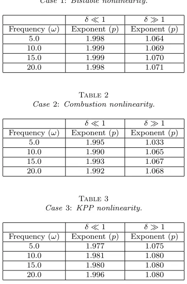
4.3. Numerical results. We are interested in testing howc∗(δ)−c0scales with
δp, especially whetherpis near 2 forδsmall andp= 1 forδ large. Using the
numer-ically calculated speedsc0 andc∗(δ), we determined the exponents pusing the least
squares method to fit a line to a log-log plot of speed versus amplitude. That is, we determined the slope of the best-fit line through the data points (log(δ),log(c(δ)−c0))
for each shear amplitude δ. For each nonlinearity we computed the exponent p for both the small amplitude and the large amplitude regimes, using a variety of frequen-cies for the time dependent shear. For the small amplitude regime, δ values range from 0.005 to 0.10 with increment 0.005. For the large amplitude regime, δ values range from 3.5 to 4.0 with increment 0.10. The exponent is observed to converge at and beyond this range ofδ.
The calculated exponents are shown in Tables 1–4 below for each nonlinearity and a sequence of temporal frequencies. These results show that with each nonlinearity, c∗(δ)−c0∼O(δ2) when the amplitude is small, andc∗(δ)∼O(δ) when the amplitude
is large. These results agree with and complement our analytical findings. In particu-lar, the growth of large amplitude bistable front speeds in shears shows an interesting contrast with the bistable front quenching (propagation failure) phenomena when either the reaction or the diffusion coefficients become strongly heterogeneous [29].
Table 1
Case1: Bistable nonlinearity.
δ≪1 δ≫1 Frequency (ω) Exponent (p) Exponent (p)
5.0 1.998 1.064
10.0 1.999 1.069
15.0 1.999 1.070
20.0 1.998 1.071
Table 2
Case2: Combustion nonlinearity.
δ≪1 δ≫1 Frequency (ω) Exponent (p) Exponent (p)
5.0 1.995 1.033
10.0 1.990 1.065
15.0 1.993 1.067
20.0 1.992 1.068
Table 3
Case 3:KPP nonlinearity.
δ≪1 δ≫1 Frequency (ω) Exponent (p) Exponent (p)
5.0 1.977 1.075
10.0 1.981 1.080
15.0 1.980 1.080
20.0 1.996 1.080
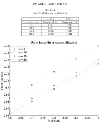
We also observe that for a fixed amplitude, the speed enhancement decreases with increasing temporal frequencyωof the shear. This can be observed clearly in the plots of the front speeds for larger amplitude shears.
Table 4
Case4: Zeldovich nonlinearity.
δ≪1 δ≫1 Frequency (ω) Exponent (p) Exponent (p)
5.0 1.991 1.038
10.0 1.991 1.045
15.0 1.993 1.046
20.0 1.992 1.047
3.6 3.65 3.7 3.75 3.8 3.85 3.9 3.95 4 0.66
0.67 0.68 0.69 0.7 0.71 0.72 0.73 0.74 0.75 0.76
Front Speed Enhancement (Bistable)
Amplitude
Front Speed c
*
ω = 5
ω = 10
ω = 15
ω = 20
Fig. 1. Comparison of bistable front speeds at moderately large amplitudes as temporal shear frequency varies;ω= 5,10,15,20.
down with increasingω and converge to a limiting value for largeω. Also the slopes are the same for differentω’s, suggesting that
c∗(δ)∼k0δ+k1(ω), δ≫1,
(4.5)
wherek0 (k1) is constant independent of (decreasing in)ω.
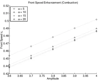
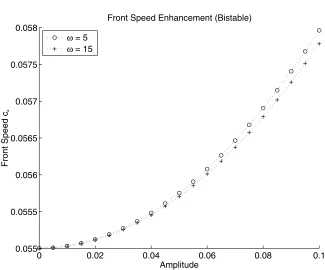
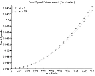
Figure 2 shows a similar comparison of combustion front speeds at the same temporal frequency values. Figures 3 and 4 illustrate the same speed slow down with increasing ω at the small shear amplitude regime. We plot only ω = 5,15, as the speed curves get much closer to each other in this regime.
3.6 3.65 3.7 3.75 3.8 3.85 3.9 3.95 4 0.43
0.44 0.45 0.46 0.47 0.48 0.49 0.5 0.51 0.52
Front Speed Enhancement (Combustion)
Amplitude
Front Speed c
*
ω = 5
ω = 10
ω = 15
ω = 20
Fig. 2. Comparison of combustion front speeds at moderately large amplitudes as temporal shear frequency varies;ω= 5,10,15,20.
5. Conclusions. Using combined analytical and numerical methods, we find that reaction-diffusion front speeds through mean zero spatially-temporally periodic shears obey robust asymptotics in both the small and large amplitude regimes. In the small amplitude regime, the enhanced speeds are proportional to shear amplitude squared, universal to all known nonlinearities. In the large amplitude regime, the en-hanced speeds scale linearly with shear amplitude, again for all known nonlinearities. In both regimes, the enhancement decreases with increasing shear temporal frequency, indicating a slowdown of front speeds under shear direction changing in time.
In future work, it will be interesting to consider spatially-temporally quasi-periodic, as well as random, shear fields and investigate efficient numerical methods that can compute large time front speeds accurately without fully resolving solutions; see [10], [6], among others.
Appendix. Traveling front existence and qualitative properties. We outline the proof of Theorem 3.1 in the case of type (4) nonlinearity. A key property is that the operator in the linear part of (2.2),
Lϕ≡ϕss+ϕy1y1+ (c∗+w(y1, τ))ϕs−ϕτ,
(A.1)
satisfiesthe strong maximum principle for (s, y1, τ)∈R1×T2 (assume without loss
of generality that ω = 1), even though locally it is parabolic. That is to say, if Lϕ≥(≤) 0 on R1×T2, where ϕ attains its maximum (minimum) at a finite point
(s0, y1,0, τ0), thenϕis identically a constant. In fact, the standard parabolic maximum
0 0.02 0.04 0.06 0.08 0.1 0.055
0.0555 0.056 0.0565 0.057 0.0575 0.058
Front Speed Enhancement (Bistable)
Amplitude
Front Speed c
*
ω = 5
ω = 15
Fig. 3. Comparison of bistable front speeds at small amplitudes as temporal shear frequency varies;ω= 5,15.
it to all τ. Based on the strong maximum principle, we apply the sliding domain method [4] to show that ϕs > 0, and 0 < ϕ < 1, and to show the uniqueness of
solutions up to a constant translation insas in [27]. The existence can be established by the method of continuation as in [30]. Let us first assume that f(u) ∈ C2. For
small δ, existence under the normalization condition maxT2ψ(0, y, τ) = θ follows
from contraction mapping principle [26]. Monotonicityϕsimplies that the linearized
operator around any solution is Fredholm and has one-dimensional kernel; hence it allows the local continuation of solution (bothϕand wave speed c∗) inδ. To ensure
the continuation to any given value ofδ, we show the closeness of continuation; namely, the limit of any sequence of solutions remains a solution. Compactness on any finite domain [−M, M]×T2 is provided by parabolicity of L. Additionally, we need to
control sat infinity. We construct upper solutions fors≤0 of the form eµsψ(y 1, τ),
whereµ >0,ψ(y1, τ)>0 uniformly in the limit so that the limiting solution decays
to zero exponentially fast ass→ −∞. Such upper solutions exist as long as the wave speedc∗<0 is uniformly bounded away from zero, which we show below. Thereafter,
f(u) ≥0 and strong maximum principle of L implies that ψ(+∞) = θ or 1. That ψ=θ is impossible, as otherwiseψwill be constant by strong maximum principle of L(contradicting its decay to zero at −∞). Existence of global solutions follows. An approximation argument takes care of less smooth reaction nonlinearities.
Now we show that c∗ is bounded away from zero. If w(y1, τ) has mean zero in
y1 for anyτ, this is done already in Proposition 3.1. Now with only space and time
mean being zero, we shall pick up additional terms to estimate. The integral
y1
0
0 0.01 0.02 0.03 0.04 0.05 0.06 0.07 0.08 0.09 0.1 0.0384
0.0386 0.0388 0.039 0.0392 0.0394 0.0396 0.0398 0.04 0.0402 0.0404
Front Speed Enhancement (Combustion)
Amplitude
Front Speed c
*
ω = 5
ω = 15
Fig. 4.Comparison of combustion front speeds at small amplitudes as temporal shear frequency varies;ω= 5,15.
whereχ0(y1, τ) andav=av(τ) are periodic. The estimate (3.5) becomes
R1×Ω
χ(F(ϕ))τ
=−
R1 −×Ω
χτF(ϕ)−
R1 +×Ω
χτG(ϕ−1)
=−
R1 −×Ω
(χ0+av′y1+χy1)y1F(ϕ)−
R1 +×Ω
(χ0+av′y1+χy1)y1G(ϕ−1)
=
R1×Ω
(χ0+χy1)ϕy1f(ϕ) +
R1×Ω
av(τ)f(ϕ)ϕτ
≤(χ0∞+χy1∞)ϕy12f(ϕ)2+av∞f(ϕ)2ϕτ2.
(A.2)
Next we boundϕτ2. Multiply (2.2) byϕτ, integrate overR1×Ω, and integrate by
parts to get
R1×Ω
(c∗+w(y1, τ))ϕsϕτ−
R1×Ω
ϕ2τ = 0,
implying via Cauchy–Schwarz inequality that
ϕτ22≤(|c0|+ 2w∞)ϕs2ϕτ2
or, in view of (3.2),
ϕτ2≤(|c0|+ 2w∞)ϕs2≤(|c0|+ 2w∞)|Ω|1/2|c∗|1/2.
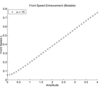
0 0.5 1 1.5 2 2.5 3 3.5 4 0
0.1 0.2 0.3 0.4 0.5 0.6 0.7 0.8
Front Speed Enhancement (Bistable)
Amplitude
Front Speed c
*
ω = 10
Fig. 5. Bistable front speeds versus amplitude at temporal shear frequencyω= 10.
Plugging (A.3) into (A.2), along with f(ϕ)2 ≤ f1∞/2|c∗|1/2|Ω|1/2, we have the
lower bound onc∗:
|c∗| ≥
χy122F(1)
|Ω| B
−1,
B= 1 2χ∞|f
′|
∞+ (1 + 2−1/2)χy1∞f1∞/2+χ∞f∞+χ0∞f1∞/2
+f1∞/2(|c0|+ 2w∞)av∞.
(A.4)
We note that the monotonicity of traveling fronts implies the attractivity of front speeds among the time dependent solutions with front initial data as in [28]. Fi-nally, we remark that uniqueness and monotonicity hold for type (1) nonlinearity, and type (1) existence for smallδ follows from [26]. With additional work, as in [5], existence for anyδand for other nonlinearities can be established. However, we shall not pursue it here.
Acknowledgments. The work was partially performed during J. X.’s visit to Institut H. Poincar´e (IHP) in October, 2002. J. X. would like to thank H. Berestycki and J.-M. Roquejoffre for their invitation and their hospitalities, as well as IHP for a visiting professorship.
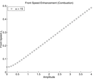
0 0.5 1 1.5 2 2.5 3 3.5 4 0
0.1 0.2 0.3 0.4 0.5
Front Speed Enhancement (Combustion)
Amplitude
Front Speed c
*
ω = 15
Fig. 6. Combustion front speeds versus amplitude at temporal shear frequencyω= 15.
REFERENCES
[1] B. Audoly, H. Berestycki, and Y. Pomeau,R´eaction-diffusion en e´coulement stationnaire rapide, Note C. R. Acad. Sci. Paris S´er. II, 328 (2000), pp. 255–262.
[2] H. Berestycki,The influence of advection on the propagation of fronts in reaction-diffusion equations, in Proceedings of the NATO ASI Conference, Cargese, France, H. Berestycki and Y. Pomeau, eds., Kluwer, Dordrecht, The Netherlands, to appear.
[3] H. Berestycki, B. Larrouturou, and P. L. Lions,Multi-dimensional travelling-wave solu-tions of a flame propagation model, Arch. Rational Mech. Anal., 111 (1990), pp. 33–49. [4] H. Berestycki and L. Nirenberg,On the method of moving planes and the sliding method,
Bol. Soc. Brasil. Mat. (N.S.), 22 (1991), pp. 1–37.
[5] H. Berestycki and L. Nirenberg,Traveling fronts in cylinders, Ann. Inst. H. Poincar´e Anal. Non Lin´eaire, 9 (1992), pp. 497–572.
[6] L.-T. Cheng and W. E,The heterogeneous multi-scale methods for interface dynamics, in Contemporary Mathematics: Special Volume in Honour of S. Osher; S. Y. Cheng, C. W. Shu, and T. Tang, eds.; AMS, Providence, RI, to appear.
[7] P. Clavin and F. A. Williams,Theory of premixed-flame propagation in large-scale turbu-lence, J. Fluid Mech., 90 (1979), pp. 598–604.
[8] P. Colella,Multidimensional upwind methods for hyperbolic conservation laws,J. Comput. Phys., 87 (1990), pp. 171–200.
[9] P. Constantin, A. Kiselev, A. Oberman, and L. Ryzhik, Bulk burning rate in passive-reactive diffusion, Arch. Ration. Mech. Anal., 154 (2000), pp. 53–91.
[10] W. E. B. Engquist,The heterogeneous multi-scale methods, Commun. Math. Sci., 1 (2003), pp. 87–132.
[11] M. Freidlin, Functional Integration and Partial Differential Equations, Ann. of Math. Stud. 109, Princeton University Press, Princeton, NJ, 1985.
[12] G. Golub and J. Ortega,Scientific Computing and Differential Equations, Academic Press, Boston, MA, 1992.
Phys. Fluids, 7 (1995), pp. 1931–1937.
[14] S. Heinze, The Speed of Travelling Waves for Convective Reaction-Diffusion Equations, Preprint 84, Max-Planck-Institut f¨ur Mathematik in den Naturewissenschaften, Leipzig, Germany, 2001.
[15] S. Heinze, G. Papanicolaou, and A. Stevens,Variational principles for propagation speeds in inhomogeneous media, SIAM J. Appl. Math., 62 (2001), pp. 129–148.
[16] A. R. Kerstein and W. T. Ashurst,Propagation rate of growing interfaces in stirred fluids, Phys. Rev. Lett., 68 (1992), p. 934.
[17] A. Kiselev and L. Ryzhik,Enhancement of the traveling front speeds in reaction-diffusion equations with advection, Ann. Inst. H. Poincar´e Anal. Non Lin´eaire, 18 (2001), pp. 309– 358.
[18] B. Khouider, A. Bourlioux, and A. Majda,Parameterizing turbulent flame speed-Part I: Unsteady shears, flame residence time and bending, Combust. Theory Model., 5 (2001), pp. 295–318.
[19] A. J. Majda and P. E. Souganidis,Large scale front dynamics for turbulent reaction-diffusion equations with separated velocity scales, Nonlinearity, 7 (1994), pp. 1–30.
[20] A. Majda and P. Souganidis, Flame fronts in a turbulent combustion model with fractal velocity fields, Comm. Pure Appl. Math., 51 (1998), pp. 1337–1348.
[21] G. Papanicolaou and J. Xin, Reaction-diffusion fronts in periodically layered media, J. Statist. Phys., 63 (1991), pp. 915–931.
[22] P. Ronney,Some open issues in premixed turbulent combustion, in Modeling in Combustion Science, Lecture Notes in Phys. 449, J. D. Buckmaster and T. Takeno, eds., Springer-Verlag, Berlin, 1995, pp. 3–22.
[23] J.-M. Roquejoffre,Stability of traveling fronts in a model for flame propagation, Part II: Nonlinear stability, Arch. Rational Mech. Anal., 117 (1992), pp. 119–153.
[24] N. Shigesada and K. Kawasaki,Biological Invasions: Theory and Practice, Oxford University Press, Oxford, UK, 1997.
[25] N. Vladimirova, P. Constantin, A. Kiselev, O. Ruchaiskiy, and L. Ryzhik,Flame En-hancement and Quenching in Fluid Flows, preprint, 2002.
[26] J. Xin,Existence and stability of travelling waves in periodic media governed by a bistable nonlinearity, J. Dynam. Differential Equations, 3 (1991), pp. 541–573.
[27] J. Xin,Existence of planar flame fronts in convective-diffusive periodic media, Arch. Rational Mech. Anal., 121 (1992), pp. 205–233.
[28] J. Xin,Existence and nonexistence of traveling waves and reaction-diffusion front propagation in periodic media, J. Statist. Phys., 73 (1993), pp. 893–926.
[29] J. Xin and J. Zhu,Quenching and propagation of bistable reaction-diffusion fronts in multi-dimensional periodic media, Phys. D, 81 (1995), pp. 94–110.
[30] J. Xin,Front propagation in heterogeneous media, SIAM Rev., 42 (2000), pp. 161–230. [31] J. Xin, KPP front speeds in random shears and the parabolic Anderson problem, Methods
Appl. Anal., to appear.
[32] V. Yakhot,Propagation velocity of premixed turbulent flames, Comb. Sci. Tech., 60 (1988), p. 191.