The impacts of land use policy on the soil erosion risk:
a case study in central Belgium
Anton J.J. Van Rompaey
a,∗,1, Gerard Govers
a,2,
Etienne Van Hecke
b, Kristine Jacobs
aaLaboratory for Experimental Geomorphology, Catholic University Leuven, Redingenstraat 16, B-3000 Leuven, Belgium bInstitute for Social and Economic Geography, Catholic University Leuven, de Croylaon 42, B-3001 Leuven, Belgium
Received 25 August 1999; received in revised form 31 January 2000; accepted 27 April 2000
Abstract
Set-aside programs of the European government have a double impact on the regional soil erosion risk in agricultural regions: (1) there is less area susceptible to soil erosion and (2) fields with a high erosion rate are preferably taken out of production resulting in a decrease of the average erosion risk. In order to quantify this double effect an inquiry among farmers in central Belgium was set up to find out which fields are preferably taken out of production. A statistical analysis pointed out that fields with a weak slope gradient, a loamy topsoil and good soil drainage have a low probability of being taken out of production. The results of the questionnaire were used to construct a transition probability map representing for each field the probability that it will be taken out of production. These transition probabilities were used to simulate the decrease in regional erosion risk for different scenarios. The outcome of these simulations suggests that there is a negative power relation between the set-aside percentage and the regional soil erosion risk. © 2001 Elsevier Science B.V. All rights reserved.
Keywords:Soil erosion; Land use changes; Set-aside; EU-CAP; Belgium
1. Introduction
The potential for surface runoff and soil erosion is very much affected by land use and cultivation. There-fore, the modelling of land use changes is important with respect to the prediction or soil degradation and its on-site and off-site consequences.
∗Corresponding author. Tel.:+32-16-32-64-11;
fax:+32-16-32-64-00.
E-mail address:[email protected] (A.J.J. Van Rompaey).
1Research Assistant of the Fund of Scientific Research (F.W.O., Flanders).
2Research Director of the Fund of Scientific Research (F.W.O., Flanders).
Many land use change studies have shown that almost all land use changes are clearly driven by hu-man activities (e.g. Turner et al., 1990; De Koning et al., 1998; Thornton and Jones, 1998). Potential land use change drivers are, for example, population growth, urbanisation, industrialisation and the devel-opment of a global economy. Regional, national or supra-national policy-makers translate these driving forces into land use regulations. Therefore, land use changes are often policy driven. However, the bio-physical conditions of the land, such as soil character-istics, climate, topography and vegetation determine to a large extent the spatial pattern of land use and land use changes. The interaction of land use change drivers with the biophysical environment takes places at the level of the land users. The importance of their
behaviour and decision rules in response to land use change drivers has only recently been recognised (Veldkamp and Fresco, 1996).
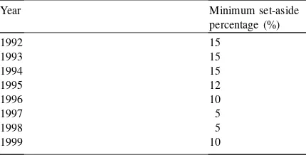
A good example of this principle is the Common Agriculture Policy of the European Union (EU-CAP). Since the reform of the EU-CAP in 1992, the support system for European farmers has thoroughly changed. The new CAP includes regulations on set-aside in order to control the level of agricultural production and to secure the income of farmers. Therefore, these EU-CAP rules can be seen as a land use change driver. The farmers are financially supported by EU relative to the area of set-aside land on their farm. Set-aside land is land that is either fallowed or used for non-food crops, e.g. energy crops. In the new support arrangements the farmer has to set aside a minimum percentage of his land, based on his area of arable land in 1991. EU changes the minimum set-aside per-centage from year to year depending on the market situation. Since 1992 the minimum set-aside percent-age has varied between 5 and 15% (see Table 1). The take-out period, during which production for agri-cultural purposes is forbidden, runs from 15 January until 31 August for a given year. Protection by vege-tation of the fallow fields with selected fallow-species is obligatory: however, the fallow species are specific for each EU-member state (Sibbesen, 1997).
As the potential for surface runoff and soil ero-sion is very much affected by land cover, these CAP-regulations potentially have a very strong impact on the average soil erosion rates in agricultural regions. A permanent vegetation cover protects the soil from direct raindrop impact, crusting and sealing which reduces the amount of surface runoff till almost zero.
Table 1
Minimum set-aside percentages since the reform of the Common Agriculture Policy of the European Union
Year Minimum set-aside
De Ploey (1989) estimated that soil erosion rates on unprotected fields may be 100–1000 times higher than on fields with permanent vegetation cover. Therefore, it may be expected that a fallow percentage of, for example, 10% will reduce the total amount of soil erosion by 10% since soil erosion on the protected fields may be reduced to 0 Mg ha−1 per year. This is indeed true if farmers select at random fields for set-aside. However, if farmers prefer to take steep and erodible fields out of production the reduction of the total erosion rate will be much higher since the average soil erosion risk of the remaining fields will be lower. Thus, insight in the decision rules that farmers use in response to the CAP-regulations is necessary to estimate the magnitude of the effects of the new policy on soil erosion in agricultural regions.
The objectives of this study are: (1) to determine what field properties do farmers take into account when selecting parcels for set-aside; (2) to model and simulate the spatial pattern of set-aside fields under different scenarios of the EU-CAP, and (3) to quan-tify the impact of different set-aside scenarios on the regional soil erosion risk.
2. Materials and methods
2.1. Landscape characteristics of the study area
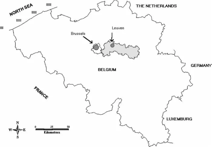
The study area (850 km2) consists of 10 municipali-ties situated in the southern part of the province Flem-ish Brabant in central Belgium (Fig. 1). The study area is a part of the Belgian loess belt, which is composed of a strongly incised plateau reaching up to 100 m above sea level. Incision of the valleys can reach 60 m (Fig. 2).
Fig. 1. Location of the study area (in grey).
(Arenosols). On the colluvium in at the footslopes Regosols can be found.
A reclassified LANDSAT satellite image allowed distinguishing different land use classes (Fig. 3; Gulinck et al., 1996). The 50% of the land in the study area consists of arable land, 17% is urban zone or infrastructure while 18% is under pasture and 13% is covered with forest.
The gradual mechanisation of the agriculture since the second world war changed the landscape structure
Fig. 2. Topography of the study area. The plateau reaches up to 100 m above sea level.
Fig. 3. Land use classes in the study area (Classified LANDSAT; Gulinck et al., 1996).
the occurrence of heavy convective showers (Vandaele and Poesen, 1995). The erosion and surface runoff on arable land on the plateau edges causes yearly prob-lems of flooding and muddy floods in the villages in the valleys (Verstraeten and Poesen, 1999). Further-more, the aquatic environment suffers from pollution because of transfers of nutrients and pesticides to the river system by leaching and surface runoff.
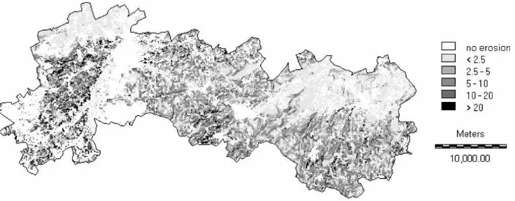
An erosion risk map (Fig. 4) of the study area was compiled by Van Rompaey et al. (2000) using the universal soil loss equation (USLE) (Wischmeier and Smith, 1978). The USLE is an empirical model that predicts the annual average, long-term water erosion rate as the product of a rainfall erosivity factor (R), a soil erodibility factor (K), a slope length factor (L), a slope steepness factor (S), a crop factor (C) and
Fig. 4. Predicted average long-term soil erosion rates in the study area (Mg ha−1 per year).
a management factor (P). Average erosion rates of more than 10 Mg ha−1per year are considered as very serious and a threat for the sustainability of the arable land. The erosion map shows that the mean annual erosion rates exceed 10 Mg ha−1 in one-third of the study area. On local hotspots soil erosion rates can exceed 50 Mg ha−1per year. The average soil erosion rate on arable land in the study area is ca. 6.0 Mg ha−1 per year.
2.2. Statistical analysis of land use patterns
2.2.1. Questionnaire
Table 2
Parcels of the 31 questioned farmers (in summer 1997) Categorya Frequency Relative frequency (%)
I 57 5.9
II 195 20.0
III 722 74.1
Total 974 100
aCategory I: fallow at the moment of the inquiry; Category II: no fallow at the moment of the inquiry but a possibly next year, and Category III: no fallow and non-considerable in the future. the study area were asked to locate their fields on aerial photographs. The farmers were asked to classify their fields in three categories: fallow at the moment of the inquiry (Category 1); no fallow at the moment of the inquiry, but a possibly in the near future (Category 2), or no fallow and none considered in the future (Category 3). In total a database of 974 fields was acquired (Table 2).
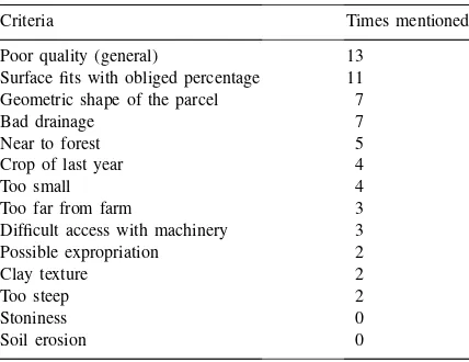
The mean criteria farmers mentioned for taking fields out of production are listed in Table 3. It is remarkable that soil erosion susceptibility is never mentioned and slope gradient only once. Drawing di-rect conclusions from Table 3 is dangerous since it is rather difficult to analyse the driving factors of one’s own decisions and behaviour. Therefore, the farmer’s responses may be rather vague (e.g. the criterion poor quality), incomplete or even biased. Moreover, for many fields farmers could not mention an exact rea-son as to why the field was taken out of production.
Table 3
Criteria for set-aside fields mentioned by farmers (results of the questionnaire)
Criteria Times mentioned
Poor quality (general) 13
Surface fits with obliged percentage 11 Geometric shape of the parcel 7
Bad drainage 7
Near to forest 5
Crop of last year 4
Too small 4
Too far from farm 3
Difficult access with machinery 3
Possible expropriation 2
Clay texture 2
Too steep 2
Stoniness 0
Soil erosion 0
It appears that the decision mechanisms of farmers with respect to set-aside are often based on personal experience and knowledge, which they find very hard to translate in objective and isolated criteria.
2.2.2. Statistical analysis of slope
A second possibility to identify possible factors re-lated to set aside is to extract some objective field characteristics and to analyse the possible differences between the two field categories (fallow and no fal-low). Therefore, statistical tests were carried out to test whether or not certain field characteristics are signifi-cantly different for fallow and non-fallow fields.
The locations of all the fields of the questioned farmers were digitised on aerial photographs resulting in a digital field-file in vector format. Digital elevation data for the study area were available from the Belgian National Geographic Institute (NGI). The dataset con-sists of regular grid data sampled every 1′′in latitude and every 2′′ in longitude from scanned topographic maps at a scale of 1:50 000. Interpolation and filtering with a low-pass filter resulted in a raster digital ele-vation model (DEM) representing the topography as a continuously varying surface. The accuracy of this DEM was evaluated with more accurate DEMs (de-rived from 1:10 000 topographic maps) for eight test areas. The overall root mean square error (RMSE) of the altimetric differences between the two DEMs is 3.1 m. The correspondence is better in the flat valleys and worse on the incised plateau. Slopes were calcu-lated using the algorithm of Zevenbergen and Thorne (1987). A regression between the calculated slopes and the slopes from the test areas provided a correction for the systematic underestimation of the slopes caused by the low resolution of the input data (Van Rompaey et al., 1999). Via an overlay of the field-file and slope map, it was possible to extract the mean slope for each field.
1972). All statistical tests were carried out using SAS procedures (SAS Institute, 1985). The procedure first tests whether the variances of the two populations are equal or not by means of an F-test. Depending on the case (equal variances or non-equal variances) the appropriate T-value is calculated which can be used to calculate the probability of the averages of the two groups (in this case the slope gradients of set-aside versus arable fields) being equal.
2.2.3. Statistical analysis of soil texture and soil drainage
Although the soils developed on the loess deposits mainly belong to the Luvisol group of the FAO soil classification (FAO, 1998), there were some variations in soil texture and soil drainage. In the northern part of the study area, the eolian deposits have a higher sand content. In the southern part of the study area, the variation in soil texture is mainly caused by outcrops of tertiary deposits that have a higher silt or clay con-tent. A soil texture map was compiled on the basis of soil cores of 1 m depth with a density of 1–2 drillings ha−1. Map purity estimates indicate that ca. 35% of the observations were classified in a textural class just above or below the correct textural class (Van Meir-venne, 1998). Soil textures were classified using the Belgian texture classification (Ameryckx et al., 1985) that does not correspond to any international classi-fication. Seven soil texture classes are distinguished: loam (A), sandy loam (P), light sandy loam (L), loamy sand (S), sand (Z), clay (E) and heavy clay (U). Soil drainage class was also mapped. Three classes were distinguished: well-drained soils, soils with a moder-ate drainage and soils with a poor drainage. Via an overlay of the field-file and the soil texture and soil drainage map, it was possible to extract for each field the soil texture class and the soil drainage class. The original texture classes were reduced to four main tex-ture classes: loam (A+P), sandy loam (L+S), sand (Z) and clay (E+U). This was done because some of the original texture classes contained very few members. This could make further analysis unreliable.
Since soil properties (texture and drainage) are qual-itative parameters, a Student t-test is not possible. Therefore, aχ2-test was used for testing whether soil properties of fallow fields are not significantly differ-ent from the non-fallow fields. Aχ2-test compares the expected frequency distribution over classes with the
observed distribution and calculates the probability of the two distributions being equal. Theχ2-value is cal-culated as follows (Wonnacott and Wonnacott, 1972):
χ2=
whereOi is the observed frequency in classi,Ei the
expected frequency in classi, andnis the number of classes.
The expected distribution of the fallow fields over the different texture classes was calculated as the to-tal distribution of all the fields in the database times the relative frequency of the fallow fields in the total amount of fields (25.9%, see Table 2). The same pro-cedure was carried out for soil drainage classes. The expected distribution over three main drainage classes (well drained, moderate drainage and poor drainage) was compared with the observed distribution.
2.3. Simulation of set-aside patterns under different scenarios
The information from the limited questionnaire was extrapolated over the whole study-area and used for simulation of the effect of different EU-CAP sce-narios. First the transition probability for each field in the study area is estimated based on its specific slope and soil characteristics. A transition probability is the probability that a field will be converted from arable land into fallow land. For a single factor (e.g. the texture class, slope class or the drainage class) the transition probability can be estimated as the relative frequency of fallow fields in that category. For exam-ple, the questionnaire results show that in the slope class 0–5, 20.5% of the fields was fallow or possibly fallow. Therefore, the transition probability for this class can be estimated as 20.5%. In the slope class 5–10% the relative frequency of fallow fields and therefore the corresponding transition probability is higher (32.5%). Such a single factor transition proba-bility can be calculated for each class of the different field characteristics (slope, texture and drainage).
However, more than one field characteristic is known. The overall transition probability can then be calculated using the theorem of Bayes
P (event|Ai∩Bi)=
P (event|Ai)∗P (event|Bi)
whereAi is theith class of variable A(e.g. the class
‘10–15%’ of slope) andBiis theith class of variable A (e.g. the class ‘sand’ of texture). This means that the probability of ‘an event’ (in our case the set-aside of a field) given conditionsAi andBi is equal to the
probability of the event under conditionAi times the
probability of the event under conditionBi divided by
the overall probability of the event. For example, the transition probability of a field for which slope and texture are known can be calculated as
P (fallow|slope class : ‘>15%’∩texture
For n factors (in this case field characteristics) the theorem can be extended.
P (fallow|Ai∩Bi ∩ · · ·Ni)
= P (fallow|Ai)∗P (fallow|Bi)∗ · · ·P (fallow|Ni) P (fallow)n−1
(4)
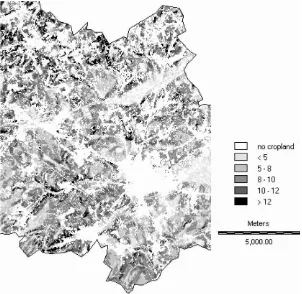
In this case the average probability for fallow (P(fallow)) is known since this is the minimum set-aside percentage of the EU-CAP (see Table 1). Using Eq. (4) the spatial pattern of transition prob-ability was calculated for a range of set-aside per-centages. An example of such a transition probability map (for a minimum set-aside percentage of 10%) is shown in Fig. 5. It is important to point out that the transition probabilities calculated using the procedure described above are independent of the distribution of observations in the sample used to derive the tran-sition probabilities. As the estimated single factor transition probabilities are the outcome of discrete events (fallow or non-fallow) their accuracy can be assessed using the theory of binomial distributions. The standard deviation of the sample mean, being the estimated single factor transition probability calcu-lated from the observed relative frequencies, can then be estimated as follows for samples having more than 20 observations (Conover, 1971)
σ = r
p×(1−p)
n (5)
wheren is the number of observations, and p is the relative frequency of transitions observed. Thus, the reliability of the transition probability is dependent only on the number of observations in each class as well as the number of transitions observed. Based on these final transition probabilities, stochastic simula-tions of possible set-aside patterns in the study area. This was done for different EU-CAP scenarios. The study area was divided in square blocks of 5 km×5 km since these spatial units correspond more or less with spatial distribution of the fields of one farmer and is therefore the level at which set-aside simulations have to be carried out. For each of these blocks set-aside volumes of 5, 10, 20 and 25% were simulated.
A simulation was carried out as follows. A field of arable land in a 5 km×5 km block was selected at random. Next a random number between 0 and 1 was chosen. This number was then compared with the transition probability of the selected field. If the random number was less than the transition probability then the field was accepted for set-aside; if not the field was left in production. This procedure was re-iterated until the desired simulated percentage of set-aside land was reached. This way of field selection implies that fields with a higher transition probability have a higher probability of being selected for set-aside.
As mentioned in the introduction fallow fields have to be protected with selected fallow crops and can thus be considered as land units with no erosion. Therefore, new soil erosion risk maps were compiled for the dif-ferent EU-CAP set-aside scenarios with soil erosion rates of 0 Mg ha−1 per year on the spots correspond-ing with a (simulated) fallow field.
3. Results and discussion
3.1. Slope of the fields
The results of thet-test are listed in Table 4. The variances of the two populations were not signifi-cantly different. The calculatedT-value of 5.53 (with 972 degrees of freedom) on the other hand has only a probability of 0.0001, which means that the mean slope of the fallow fields was significantly higher than the mean slope of the non-fallow fields.
Fig. 5. Land use transition probabilities (%) from cropland to fallow land (set-aside percentage=10%).
farmers make decision about set-aside. However, only 2 out of the 31 farmers that were questioned explicitly mentioned the slope gradient as a decision criterion (Table 3) This is a problem that already has been
Table 4
Slope distribution of fallow and non-fallow fields Category I+
Category IIa
Category IIIa
No. of observations 252 722
Mean slope gradient (%) 5.84 4.67 S.D. of slope gradients 3.02 2.86
F-value 1.12
P>F 0.26
T-value 5.53
P>T 0.0001
aCategory I: fallow at the moment of the inquiry; Category II: no fallow at the moment of the inquiry but possibly next year and Category III: no fallow and non-considerable in the future.
recognised by many researchers in psychology and related social sciences (Austin et al., 1998a,b; Hengs-dijk, 1998; Van Ittersum, 1998). In this particular case, farmers probably do not see slope gradient as a sep-arate and isolated field property but incorporate it in the more general field property ‘good or poor quality’.
3.2. Soil texture
Table 5
Expected versus observed distribution of fallow fields over soil texture classes
The null-hypothesis ‘set-aside fields have the same distribution over different soil drainage types’ was tested by means of a χ2-test. The results are listed in Table 6. The analysis confirmed that the null-hypothesis can be rejected. Thus, wet fields are much more likely to be taken out of production than fields with good soil drainage.
3.4. Impact of set-aside on the soil erosion risk
The former statistical analysis shows that slope gradient, soil texture and soil drainage do have a significant influence on the choices made by farm-ers. Apparently steep fields with a sandy or clay soil
Table 7
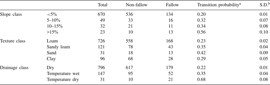
Transition probabilities for field characteristics
Total Non-fallow Fallow Transition probabilitya S.D.b
Slope class <5% 670 536 134 0.20 0.01
5–10% 49 33 16 0.32 0.07
10–15% 32 21 11 0.34 0.08
>15% 23 10 13 0.56 0.10
Texture class Loam 726 558 168 0.23 0.02
Sandy loam 121 78 43 0.35 0.04
Sand 31 18 13 0.42 0.09
Clay 96 68 28 0.29 0.05
Drainage class Dry 796 617 179 0.22 0.01
Temperature wet 147 95 52 0.35 0.04
Temperature dry 31 10 21 0.68 0.08
aSingle factor transition probability. bCalculated using Eq. (5).
Table 6
Expected versus observed distribution of fallow fields over soil drainage classes
Table 8
Decrease in soil erosion risk as a consequence of set-aside Minimum
set-aside %
Average erosion rate fallow fieldsa (Mg ha−1per year)
Average soil erosion rate remaining arable fields (Mg ha−1 per year)
Total amount of soil erosion in the study areab (Mg per year)
0 – – 408 000
5 33.1 9.6 367 400
10 25.6 9.1 328 900
15 22.2 8.6 296 200
20 20.3 8.2 265 200
aThe listed erosion rates are theoretical. Since these fields are protected the real erosion rate is reduced to 0 Mg ha−1per year. bThe total surface area is 850 km2.
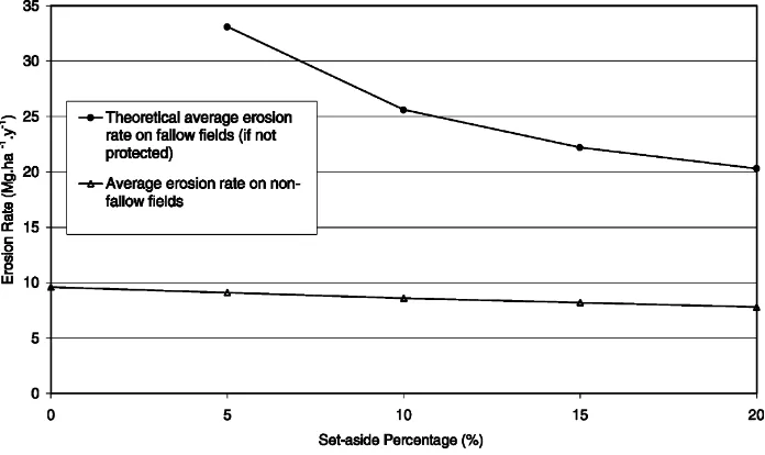
simulation show that there is lowering of the average soil erosion rate of the remaining arable fields when set-aside is introduced. This is due to the fact that farmers tend to take out of production the steepest fields. The preference for fields with sand and clay soils, on the other hand, has a negative effect on the average erosion risk of the remaining fields since these texture are slightly less erodible than the loamy soils. In Fig. 6 the ‘theoretical average erosion rate’ of fallow fields (i.e. the erosion rate of the fallow fields if they were not protected with fallow crops) is plotted against the fallow percentage. It appears that the theoretical average erosion rate of the fields that are taken out of production is much higher than the
Fig. 6. Average soil erosion rate on non-fallow fields. The erosion rates were calculated with the USLE. The set-aside patterns were simulated.
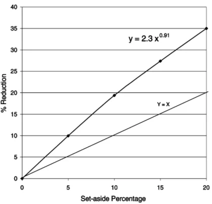
Fig. 7. Reduction of the total soil erosion in the study area. The erosion rates were calculated with the USLE. The set-aside patterns were simulated.
production is lower for higher set-aside percent-ages, the decrease of the average erosion rate of the non-fallow fields is dropping as well.
Combining the decreasing erosion rate on the remaining arable fields with the linear decrease of the area arable land results in an faster than linear decrease of the erosion rate with increasing set-aside percentages as is illustrated in Fig. 7. The observed trend can be described with a power function of the form
D=aSb (6)
whereD is the decrease in soil erosion in the study area,S the set-aside percentage, andaandb are the regression coefficients.
4. Conclusions
Based on the statistical analysis of the results of an questionnaire, the decision mechanisms of the farm-ers and their interaction with the physical environment was simulated for different scenarios of the set-aside programs of the EU-CAP. The results of the ‘objective’ statistical analysis were somewhat in contradiction with the ‘subjective’ criteria that farmers mentioned
for taking fields out of production. The statistical anal-ysis pointed out that slope is a very significant crite-rion while this factor is almost completely absent in the farmer’s answers to the questionnaire. This sug-gests that the results of farmer’s questionnaires should be used with care when studying decision procedures. This has also been observed in other studies trying to model the effectiveness of agricultural policies on farmer’s behaviour using psychological, social and economic variables (Austin et al., 1998a,b; Hengsdijk et al., 1998; Van Ittersum et al., 1998).
The relative reduction in total soil erosion in the re-gion is far more important than the relative reduction in arable land. This is due to the fact that steep fields are preferentially selected by farmers for set-aside. The results of the set-aside simulations also show that the decrease of total soil erosion in the region with in-creasing set-aside percentage is degressive. This trend is explained by the combination of (i) the reduction of the total area of arable land, and (ii) a reduction of the average soil erosion rate on the remaining arable land. Neglecting the farmer’s decision criteria would lead to a serious underestimation of the effects of the EU-CAP rules on the regional soil erosion risk in the study area (Fig. 7).
The positive effect of set-aside on the decrease in soil erosion risk might be taken into consideration by the EU-CAP as a soil conservation measure. As set-aside may help to control the high costs for the community related to the negative off-site effects of soil erosion, a policy encouraging set-aside might be maintained even if this is not required by the price sit-uation of grain crops. In the US similar programs are already running. According to Brady and Weil (1999, Chapter 17, p. 717) a major part (about 60%) of the reduction in soil erosion experienced in the US since 1982 is due to the conservation reserve program (CRP) that pays farmers to shift some land from crops to grasses and forest.
Acknowledgements
Fund for Scientific Research of Flanders is gratefully acknowledged.
References
Ameryckx, J., Verheye, W., Vermeire, R., 1985. Bodemkunde. J. Ameryckx, Gent, 255 pp.
Austin, E.J., Willock, J., Deary, I.J., Gibson, G.J., Dent, J.B., Edward-Jones, G., Morgan, O., Grieve, R., Sutherland, A., 1998a. Empirical models of farmer behaviour using psycho-logical social and economic variables. Part I: linear modelling. Agric. Syst. 58 (2), 203–224.
Austin, E.J., Willock, J., Deary, I.J., Gibson, G.J., Dent, J.B., Edward-Jones, G., Morgan, O., Grieve, R., Sutherland, A., 1998b. Empirical models of farmer behaviour using psycholo-gical social and economic variables. Part II: nonlinear and expert modelling. Agric. Syst. 58 (2), 225–241.
Brady, N.C., Weil, R.R., 1999. The Nature and Properties of Soils. Prentice-Hall, Englewood Cliffs, NJ.
Conover, W.J., 1971. Practical Nonparametric Statistics. Wiley, New York.
De Koning, G.H.J., Veldkamp, A., Fresco, L.O., 1998. Land use in Ecuador: a statistical analysis at different aggregation levels. Agric., Ecosyst. Environ. 70, 231–247.
De Ploey, J., 1989. Erosional systems: a perspectives for erosion control in European löss areas. Soil Technol. Ser. 1, 93–102. Desmet, P.J.J., Ketsman, W., Govers, G., 1999. An evaluation of the
effects of changes in field size and land use on soil erosion using a GIS-based USLE approach. In: Craglia, M., Onsrud, H. (Eds.), Geographic Information Research: Transatlantic Perspectives. Taylor & Francis, London.
FAO, 1998. World Reference Base for Soil Resources. FAO World Soil Resources Reports, No. 84, FAO, Rome, Italy, 88 pp. Goossens, D., 1993. The Belgian löss deposits: an overview.
Geomorphological processes in the Belgian löss belt. Excursion Guide: Memorial Symposium Prof. J. De Ploey. Experimental Geomorphology and Landscape Ecosystem Changes, 24 March 1993, Leuven, pp. 5–10.
Gulinck, H., Janssens, K., Sanders, J., 1996. Digitale versie van de Bodemgebruikskaart Vlaanderen. OC-GIS Vlaanderen. Hengsdijk, H., van Ittersum, M.K., Rossing, W.A.H., 1998.
Quantitative analysis of farming systems for policy formulation: development of new tools. Agric. Syst. 58 (3), 381–394.
SAS Institute, 1985. SAS Users Guide: Statistics, 5th Edition. SAS Institute Inc., Cary, NC, 956 pp.
Sibbesen, E., 1997. Set-aside and land-use regulations with relation to surface runoff in Finland, Denmark and Scotland, Belgium, France and Spain. SP-report No. 14, Danish Institute of Agricultural Science.
Thornton, P.K., Jones, P.G., 1998. A conceptual approach to dynamic agricultural land-use modelling. Agric. Syst. 57 (4), 505–521.
Turner, B.L., Clark, W.C., Kates, R.W., Richards, J.F., Matthews, J.T., Meyer, W.B., 1990. The Earth as Transformed by Human Action. Cambridge University Press, Cambridge.
Vandaele, K., Poesen, J., 1995. Spatial and temporal patterns of soil erosion rates in an agricultural catchment, Central Belgium. Catena 25 (1/4), 213–226.
Van Ittersum, M.K., Rabbinge, R., van Latesteijn, H.C., 1998. Exploratory land use studies and their role in strategic policy making. Agric. Syst. 58 (3), 309–330.
Van Meirvenne, M., 1998. Predictive quality of the Belgian soil survey information. Pedologie Themata. J. Belgian Assoc. Soil Sci. 5, 21–29.
Van Oost, K., Govers, G., Desmet, P., 2000. Evaluating the effects of changes in landscape structure on soil erosion by water and tillage. Landscape Ecol. 15, 579–591.
Van Rompaey, A., Govers, G., Baudet, M., 1999. A strategy for controlling error in distributed environmental models by aggregation. Int. J. GIS 13 (6), 577–590.
Van Rompaey, A., Govers, G., Waumans, T., 2000. Een regionale bodemerosierisicokaart voor Vlaanderen. @WEL No. 3, 6 pp. (http://www.wel.be).
Veldkamp, A., Fresco, L.O., 1996. CLUE: a conceptual model to study the conversion of land use and its effects. Ecol. Model. 85, 253–270.
Verstraeten, G., Poesen, J., 1999. The nature of small-scale flooding, muddy floods and retention pond sedimentation in central Belgium. Geomorphology 29 (3/4), 275–292. Wischmeier, W.H., Smith, D.D., 1978. Predicting rainfall erosion
losses: a guide to conservation planning. USDA Agriculture Handbook 537.
Wonnacott, T.H., Wonnacott, R.J., 1972. Introductory Statistics. Wiley, New York.