TWO METHODS FOR SELF CALIBRATION OF DIGITAL CAMERA
Aparajithan Sampatha ,Donald Moea, Jon Christophersona
aSGT, Inc1, U.S. Geological Survey (USGS) Earth Resources Observation and Science (EROS) Center, Sioux Falls, SD 57198 USA –(asampath, dmoe,jonchris)@usgs.gov
KEY WORDS: Photogrammetry, Rectification, Bundle, Camera, Geometric.
ABSTRACT:
Photogrammetric mapping using Commercial of the Shelf (COTS) cameras is becoming more popular. Their popularity is augmented by the increasing use of Unmanned Aerial Vehicles (UAV) as a platform for mapping. The mapping precision of these methods can be increased by using a calibrated camera. The USGS/EROS has developed an inexpensive, easy to use method, particularly for calibrating short focal length cameras. The method builds on a self-calibration procedure developed for the USGS EROS Data Center by Pictometry (and augmented by Dr. C.S Fraser), that uses a series of coded targets. These coded targets form different patterns that are imaged from nine different locations with differing camera orientations. A free network solution using collinearity equations is used to determine the calibration parameters. For the smaller focal length COTS cameras, the USGS has developed a procedure that uses a small prototype box that contains these coded targets. The design of the box is discussed, along with best practices for calibration procedure. Results of calibration parameters obtained using the box are compared with the parameters obtained using more established standard procedures.
1. INTRODUCTION
1.1 General
For any photogrammetric project, an accurate knowledge of the sensor/camera’s interior orientation parameters is necessary. In this research, we shall present two methods used by the USGS to determine these parameters for small and medium format digital cameras. The first method, developed by Pictometry (augmented by Dr C.S. Fraser), uses a series of coded targets on a cage. The coded targets are placed on the cage in three different planes, which allows for a robust calibration procedure. The second method describes the development of a method whereby the coded targets are pasted on a small prototype box. The importance of calibrating a camera used for photogrammetric purposes cannot be overstated. The interior orientation parameters of a camera help in determining the exact path of a ray of light that enters a camera, at the time of exposure. The main interior orientation parameters are the focal length of the lens and the location of the principal point of symmetry. The knowledge of the deviation of the light ray from a straight line, described by polynomial coefficients, is also important. This deviation is termed lens distortion, and the polynomial coefficients are termed lens distortion parameters. Photogrammetric projects can be executed without a thorough knowledge of the calibration parameters too. However, these would require a very dense network of control points that will render these projects prohibitively expensive.
1.2 Camera calibration methods
Camera calibration methods preferred by photogrammetrists can be categorized broadly into three classes, In-situ calibration, calibration using precise multi-collimator instruments and self-calibration.
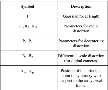
Symbol Description
f Gaussian focal length
K1, K2, K 3 Parameters for radial distortion
P1, P2 Parameters for decentering distortion
B1, B2 Differential scale distortion (for digital cameras)
,
xp y p Position of the principal point of symmetry with respect to the array pixel
frame.
Table 1. List of interior orientation parameters
1.2.1 In-situ calibration: In-situ methods require In-situ calibration methods require an area (a calibration range) with a very dense distribution of highly accurate control points. The control points in the calibration range should be well distributed in the horizontal, as well as in the vertical direction. The in-situ method requires aerial imagery over a calibration range. A rigorous least squares block adjustment based on the co-linearity equations, augmented by equations modelling radial and decentring distortion (Eq. 5) can generate accurate calibration parameters. On many occasions, these calibration procedures are used to validate photogrammetric data (Cramer and Haala, 2009), or validate/augment the calibration
parameters determined in the laboratory. The calibration range should be maintained periodically, and may include re-survey of the control points, making sure they are undisturbed etc.
1.2.2 Precision multi-collimator instruments: The USGS operates a multi-collimator calibration instrument located at Reston, Virginia, USA (Light, 1992). The instrument is used to calibrate film based cameras, and while digital cameras are increasingly used, there are a number of photogrammetric companies that still employ film cameras. The aerial camera is calibration parameters (Eq. 5).
1.2.3 Self calibration: Self calibration uses the information present in images taken from an un-calibrated camera to determine its calibration parameters (Fraser, 1997; Fraser 2001; Remendino and Fraser, 2006; Strum, 1998). Methods of self calibration include generating Kruppa equations (Faugeras et. al., 1992), enforcing linear constraints on calibration matrix (Hartley, 1994), a method that determines the absolute quadric, which is the image of the cone at a plane at infinity (Triggs. While there are many techniques employed by researchers (Hartley, 1994; Faugeras et al., 1992), most of these do not find solutions for distortion and principal point, as they are not considered critical for Computer Vision. On the other hand, for photogrammetrists, these are critical parameters necessary to produce an accurate product at a reasonable price.
In this research, self-calibration techniques are used to determine camera calibration parameters. Section 2 provides a brief theoretical framework for calibration. It goes on to discuss the design of two methods for self calibration used at the USGS, and describes the experimental set-up. It introduces an inexpensive method for calibrating small and medium format digital cameras, with short focal length. Section 3 analyses the results of calibration, and compares the results obtained from the two methods described in Section 2. Section 4 presents the conclusions and discusses future work.
2. CALIBRATION METHODOLOGY
2.1 Theoretical basis
The self calibration procedure described in this research is based on the least squares solution to the photogrammetric resection problem. The well known projective collinearity equations form the basis for the mathematical model.
In Eq. 1, (x ,y) are the measured image coordinates of a feature and (xp, y ) are the location of the principle point of the lens, p
in the image coordinate system, f’ refers to the focal length and
interested in characterizing the radial distortion and de-centring distortion. Radial distortion displaces the image points along the radial direction from the principal point (Mugnier et al., 2004). The distortion is also symmetric around the principal point. The distortion is defined by a polynomial (Brown, 1966; Light, 1992).
The (x,y) components of the radial distortion are given by:
r
The second type of distortion is the decentring distortion. This is due to the displacement of the principle point from the centre of the lens system. The distortion has both radial and tangential components, and is asymmetric with respect to the principal point (Mugnier et al., 2004). The components of de-centring distortion, in the x-y direction are given by
) direction is also incorporated
The final mathematical model is a result of adding Eqs. 3 and 4 and 5 to the right hand side of Eq.
2.2 Experimental set-up for cage based self calibration
30 FEET WIDE
7
0
FE
E
T
L
ON
G
14 FEET WIDE
5
4
FE
E
T
L
ON
G
CEILING HEIGHT INSIDE CENTER BOX
12 FT, 9 IN CEILING
HEIGHT ON OUTSIDE
RING 10 FT, 7 IN
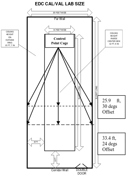
EDC CAL/VAL LAB SIZE
8 FT
8
FT
DOUBLE DOOR Far Wall
Corridor Wall
Figure 1. Layout of the calibration lab and the calibration cage
The camera calibration facility is located at the USGS’s Earth Resources Observation and Science (EROS) Data Center in Sioux Falls, South Dakota. Fig. 1 shows the position of the calibration cage, with respect to the room. Also shown are some of the positions for locating the cameras. The cage consists of three parallel panels. Each panel has a number of circular retro-reflective targets (dots), and a few coded targets (Fig 2a). The coded targets are so referred because the pattern of the placement of the individual circular dots that make up these targets is unique (Fig. 2b). Each coded target has five dots that are positioned in the same relative orientation as the red lines shown in Fig. 2(b). The intersection of the red lines is taken as the centre of the coded target.
For the calibration procedure, the camera lens is always focussed at infinity (unless the camera is used for close range purpose, in which case the focus is fixed at the specified distance). The choice of the distance of the camera from the front panel of the cage depends on the focal length of the camera, and the depth of focus that has been selected. Once the camera-cage distance is fixed, three angular positions from the centre of the front panel of the cage are selected, keeping in mind the optimal angles for convergent photography, and the limitations imposed by the dimensions of the calibration room. Ideally, the angular positions will be close to what is shown in Fig 1. Once the images are captured, they are processed using software called Australis (Fraser, 2001). Australis uses a free network method of bundle adjustment. It recognizes the patterns in the coded targets and calculates their centre.
(a) 3D Calibration cage
(b) Coded target (c) Circular target
Figure 2. (a) Image of the calibration cage, with three panels (b) the pattern in a coded target and (c) the individual circular
target
The coded target centre is not the actual centroid of the individual target dots, but determined in a manner shown in Fig. 2(b). The software requires at least four coded targets in each image that are common with other images. It uses the targets to determine the initial relative orientation of the camera at all the exposure stations. It then uses the circular targets to determine a free network least squares bundle adjustment solution of Eq. 5. Since it is a free network solution, the least squares iteration converges easily, and a relative measure of the geometry of the system (the lens, camera, and the targets) is obtained.
2.3 Camera self calibration using a box
With the ever increasing use of small platform based digital photogrammetry (such as UAV, etc.) for aerial mapping, the USGS developed a self-calibration procedure for small format cameras that does not require establishing a large calibration cage. Instead, a smaller rigid box that can be easily designed and constructed is used. The current design of the box is as shown in Fig. 4(a). The box is designed such that its dimensions are approximately 24 inches at the top (outer edge) and 12 inches at the bottom (inner). The inner walls of the box are not vertical, but are sloping at approximately 30 degrees. A scaled down series of coded targets are pasted on all the interior surfaces of the box. The design takes advantage of the simplicity of the free network bundle adjustment solution that requires no outside control structure.
Control Point Cage 12Wx10Hx8
25.9 ft, 30 degs Offset
33.4 ft, 24 degs Offset
Coded target centre
(a) (b)
Figure 4(a). A rigid box design for calibration of small format cameras and (b) another design with an increased number of
targets
A smaller box (Fig. 4(b)) with an increased number of coded targets and circular targets was also designed for use with cameras with a very small field of view. For calibration photography, the optic axis of the camera is usually kept parallel to the inclined interior walls of the box. Three images are obtained from each side, and one image is obtained from each of the four corners, which results in a total of sixteen images. The images are alternatively taken in portrait and landscape modes. However, for cameras to be used with the smaller box, the photography is along parallel axis, mimicking the collection of vertical aerial images for a photogrammetric project. For a stable solution, as many targets as possible are obtained from the corners of the camera lens.
3. RESULTS AND ANALYSIS
Two cameras are analysed in this paper. The first one is a Nikon D1x digital single lens reflex (SLR) camera with a 20mm focal length lens (Nikkon AF) was used for this research. F # of 8 was chosen for calibrating with the cage as target, and f # of 22 was chosen for calibrating with the box as the target. The second camera is also a Nikon D70 camera with a 70mm-180mm lens. This camera was used to make photogrammetric measurements on the Fragment C of the Antikythera mechanism (Evans et. al., 2010). The camera’s (hence called Puget Sound camera) focal length was fixed at around 70mm by the researchers working to measure the Antikythera. However, to determine the exact focal length and the geometric distortions due to the lens, the Puget Sound camera and lens were sent to the USGS EROS.
3.1 Results
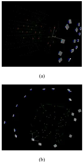
The results of the experiments are shown in Fig2. 6-8 and Tables 2-3. A total of 15 images were of the cage taken for use in the calibration software. Usually, only nine images are used. However, in this case 15 images were required to completely cover all the targets. The free network bundle adjustment solution is graphically displayed in Fig 7 (a). In a similar manner, the hyperfocal distance for the calibration using the box was calculated at 1 ft. A total of 20 images were obtained for the box. The free network solution is graphically shown in Figure 7 (b). The green dots in Fig. 6 represents a circular target (Fig 2c), while the orange lines represent the coded target patterns (Fig. 2b).
(a)
(b)
Figure 6. Graphical representation of the bundle adjustment solution for (a) Cage and (b) Box based camera calibration
.
Calibration parameters
Calculated values from
cage
Calculated values from
box
Focal length 20.601 20.603
Principle point location
p
x 0.056 mm 0.064 mm
p
y -0.020 mm -0.019mm
Radial distortion coefficients
K1 2.781e-004 2.74196e-004
K2 -4.996e-007 -4.1747e-007
K3 9.139e-011 -1.5359e-011
De-centring distortion coefficients
P1 -6.173e-007 2.989e-007
P2 8.341e-006 2.637e-005
Scaling elements
B1 8.1521e-005 1.5082e-005
B2 -1.0153e-005 9.6088e-006
Table 2 Camera calibration parameters
Table 2 shows the solutions to the bundle adjustment and the calibration parameters obtained from the two experiments. Table 2 lists the calibration parameters that were obtained as a part of the bundle adjustment solution. Fig. 7 shows the plots of radial distortion obtained while using the cage (Fig. 7a) and while using the box (Fig. 7b)
(a)
(b)
Figure 7. Radial distortion plots showing the distortion (Y-axis, µm) as a function of distance (X-axis, mm) from the principal point for results of camera calibration obtained from (a) Cage and (b) Box. The plots are obtained from Australis software
(a)
(b)
Figure 8. Decentring distortion plots showing distortion (Y-axis, µm), against radial distance (X-(Y-axis, mm) for results of camera calibration obtained from (a) Cage and (b) Box. The
plots are obtained from Australis software
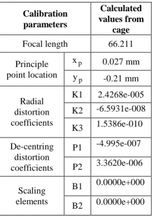
Fig. 8a and Fig.8b show the results for decentring distortion obtained using the cage and the box, respectively. The results for the Puget Sound camera are shown in Table 3. In this case, the smaller box was used, because it had a very small field of view. Almost 135 images were used to arrive at the solution.
Calibration parameters
Calculated values from
cage Focal length 66.211
Principle point location
p
x 0.027 mm
p
y -0.21 mm
Radial distortion coefficients
K1 2.4268e-005
K2 -6.5931e-008
K3 1.5386e-010
De-centring distortion coefficients
P1 -4.995e-007
P2 3.3620e-006
Scaling elements
B1 0.0000e+000
B2 0.0000e+000
Table 3 Camera calibration parameters for the Puget Sound Camera
3.2 Analysis
The results from the bundle adjustment are initially calculated in the camera pixel space. The results are converted into real world coordinates by using the pixel size as the scale factor. This replaces the fiducial marks used in film cameras. Therefore, each pixel (or the average pixel) is considered to the equivalent of the measurements from the fiducial mark. The results of the two calibration procedures indicate that the parameters are close to being identical (Table 2). The charts in Fig. 7a and 7b also show the similar results. However, in our experiments, we found that the results start varying if the camera is positioned too close to the targets. This observation seems consistent with previously reported studies on close range photogrammetric camera calibration (Brown, 1971). However, more analysis needs to be done for anything conclusive. Table 3 lists the results for the results from the Puget Sound camera. The field of view of the Puget Sound camera was too small to be used with the cage or the box described above. Hence, an even smaller box with a more dense distribution of coded and circular targets was constructed. The results indicate a large principal point offset, as well as a higher than usual deviation from the nominal focal length of 70mm. Since the box as a calibration target is meant for small format short focal length cameras, the distance between the targets and the cameras should be close enough so that the software is able to recognize the targets. The size of the targets, therefore, needs to be selected accordingly.
4. CONCLUSIONS
In this research, two methods of camera calibration that are used at the USGS EROS at Sioux Falls, South Dakota, USA were presented. The camera calibration lab is housed primarily to calibrate medium format digital cameras, with a focal length range between 20-120mm. The main calibration method uses the principles of self calibration and bundle adjustment on coded targets located on an aluminium cage. A second method to perform calibration was presented. This method used a scaled
Both the methods involve taking images of the targets from different camera locations and orientations. It was shown that the solutions camera calibration parameters obtained from both the methods are close to each other. The same time the approach using the box yields promising results and can be used for verification of the calibration parameters.
References:
Brown, D.C., 1996. Decentering distortion of lenses. Photogrammetric Engineering, 32(3):444– 462.
Brown, D.C., 1996. Close-range camera calibration. Photogrammetric Engineering, 37(8):855– 866, August 1971
Cramer, M., Haala, N. 2009. DGPF project: Evaluation of digital photogrammetric aerial bases imaging systems— overview and results from the pilot centre. In Proceedings of the ISPRS Hannover Workshop, Hannover, Germany, June 2-5, 2009.
Evans, J., Carman C. C., Thorndike, A.S, 2010. Solar anomaly and planetary displays in the Antikythera mechanism. Journal for the history of astronomy, xli (2010), 1–39.
Faugeras, O., Luong, Q.T. and Maybank, S., 1992. Camera selfcalibration: Theory and experiments. ECCV'92, Lecture Notes in Computer Science, Vol. 588, Springer-Verlag, pp. 321-334
Fraser, C.S., 1997. Digital camera self-calibration. ISPRS Journal of Photogrammetry & Remote Sensing 52, pp. 149– 159, 1997.
Fraser, C.S., 2001. Australis: software for close-range digital photogrammetry users manual.
Hartley, R., 1994: Euclidean reconstruction from uncalibrated views. In Applications of Invariance in Computer Vision, Mundy, Zisserman and Forsyth (eds.), Lecture Notes in computer Science, Vol. 825, Springer-Verlag, pp. 237-256
Remondino, F., Fraser, C.S., 2006. Digital camera calibration methods: considerations and comparisons. IAPRS volume XXXVI, part 5, Dresden 25-27 September 2006
Lee, G.Y.G. ,2004. Camera calibration program in the United States: past, present and future. In Post-Launch Calibration of Satellite Sensors, ISPRS Book Series, Vol. 2, A.A. Balkema Publishers, New York.
Light, D.L.,1992. The new camera calibration system at the U.S.Geological Survey. Photogrammetric Engineering and Remote Sensing, 58(2):185–188.
Mugnier, C.J., Forstner, W., Wrober, B., Padres, F., Munjy, R., 2004. The mathematics of photogrammetry. In Manual of Photogrammetry, Fifth edition. Pp. 181-316.
Strum., P., 1998. A case against Kruppa’s equations for camera self-calibration. IEEE International conference on image processing, Chicago, Illinois, pp. 172-175.
Triggs, B., 1997. Autocalibration and the absolute quadric,CVPR, pages 609–614, Puerto Rico, June 1997.
DISCLAIMER
Any use of trade, product, or firm names is for descriptive purposes only and does not imply endorsement by the U.S. Government.