FOOTPRINT MAP PARTITIONING USING AIRBORNE LASER SCANNING DATA
B. Xiong a, , S. Oude Elberink a, G. Vosselman a
a
ITC, University of Twente, the Netherlands - (b.xiong, s.j.oudeelberink, george.vosselman)@utwente.nl
Commission III, WG III-2
KEY WORDS: Footprint map decomposition, ALS data, 3D building modelling, LoD1, LoD2
ABSTRACT:
Nowadays many cities and countries are creating their 3D building models for a better daily management and smarter decision making. The newly created 3D models are required to be consistent with existing 2D footprint maps. Thereby the 2D maps are usually combined with height data for the task of 3D reconstruction. Many buildings are often composed by parts that are discontinuous over height. Building parts can be reconstructed independently and combined into a complete building. Therefore, most of the state-of-the-art work on 3D building reconstruction first decomposes a footprint map into parts. However, those works usually change the footprint maps for easier partitioning and cannot detect building parts that are fully inside the footprint polygon. In order to solve those problems, we introduce two methodologies, one more dependent on height data, and the other one more dependent on footprints. We also experimentally evaluate the two methodologies and compare their advantages and disadvantages. The experiments use Airborne Laser Scanning (ALS) data and two vector maps, one with 1:10,000 scale and another one with 1:500 scale.
1. INTRODUCTION
1.1 Motivation
Height data is necessary for reconstructing 3D building models. The height data could be one or several of them including DSM (Lafarge et al., 2008; Vallet et al., 2011), photogrammetric point cloud (Xiong et al., 2014a), lidar points (Kada and McKinley, 2009; Lafarge and Mallet, 2012; Sohn et al., 2008; Xiong et al., 2014b), and SAR (Thiele et al., 2010). On the other hand, the footprint maps of buildings are used as well (Kada, 2009; Oude Elberink et al., 2013; Suveg and Vosselman, 2004). The reasons to use footprint maps are twofold. First, the footprint maps provide accurate building boundaries for inferring the inner structure. Second, the 3D building models is an extension of 2D maps. Most authorities and users want the two data sets to have consistent outlines on the ground level. While we have already spent a big effort to maintain and update 2D maps, it is reasonable and easier to require the newly made 3D building models to match with the 2D maps.
A building often has multiple parts that are separated by height jumps. Each building part can be reconstructed independently and the reconstruction complexity will be decreased significantly(Haala and Kada, 2010). For example, in the model-driven method, the searching of building primitives are decreased to the local area of one partition (Kada and McKinley, 2009; Oude Elberink and Vosselman, 2009). On the other hand, the partition improves model details with little costs. In the OGC definition (Kolbe et al., 2009), an LoD1 building model is just a block that extrudes the footprint map onto a certain height. This building model is too coarse to satisfy many applications like the calculation of volume, shadow and line-of-sight. While it is still challenging to reconstructing LoD2 models fully automatically. A simple trade-off is to decompose a building footprint into parts and model each part as a block, see Figure 2. The extended LoD1 model is called LoD1+, and is a good trade-off between LoD1 and LoD2 models.
Corresponding author
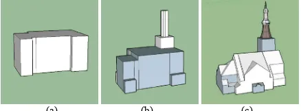
(a) (b) (c)
Figure 1. A building in different Level of Details (LoD). (a) The LoD1 model; (b) the LoD1+ model; (c) the LoD2 model. The extended LoD1+ models is a good trade-off between LoD1 and LoD2 models.
Map partitioning has been done by inferring from maps only or by combining maps with height data. Footprint maps give hints about inner structures thereby some parts can be derived with the footprint only. However many parts, especially the parts not touching the footprint, can only be inferred by taking height data into account. But even when the height data is applied, many problems need to be considered, including detection of all partitions, constraining of dominant directions, and maintenance of small structures.
In this paper, we analyse difficulties in map decomposition and define minimum requirements that we need to meet for the decomposition task. We thereby introduce two novel map decomposition methodologies. Both use the footprint map and lidar point cloud. The lidar points are decomposed into layers according to their height differences. The first one derives contours for roof layers and snaps them to footprint maps. The second one detects steps edges between roof layers and combine them with footprint maps for decomposition.
1.2 Related Works
Haala et al. (2006) assume that all buildings have one or more dominant directions with small extensions, and assume that all ISPRS Annals of the Photogrammetry, Remote Sensing and Spatial Information Sciences, Volume III-3, 2016
partitions can be derived from footprint outlines. The dominant directions are derived by averaging closely parallel outlines. Small extrusions are merged to those dominant directions, thereby the footprint is generalized. Partitioned cells are achieved by extending and intersecting all outlines. Haala et al. (2006) take all partitioned cells as final result without merging. Because some of those cells may be actually belonging to one building part, Commandeur (2012) merge them into groups by combining lidar point segments. As the footprints are generalized, they do not keep consistent. This type of methods only infers partitions from footprint map, the parts that are fully inside the building cannot be detected.
Vosselman and Suveg (2001) observe that footprint maps are not enough to derive building partitioning. They first detect jump edges between roof components that are discontinuous over heights. The jump lines are then used to split footprint maps by combining with concave line extensions of footprint maps. Those partitioned cells are merged to building parts by grouping cells that have same lidar segments. The problem is that only one step line is detected from a pair of adjacent building parts. In fact, in many cases, they have two or more step lines, resulting badly partitioned building parts. Meanwhile, because the boundary points are usually noisy and incomplete, the partition lines are not precise, and do not match well with footprint corners.
In order to find building parts inside footprint maps, Vallet et al. (2011) use push-broom lines instead of step edges. By sweeping all dominant directions across the building, a set of candidate partition lines can be achieved. The one whose buffer area with largest DEM difference is kept as a partition line. The push-broom lines follow dominant directions of the footprint to avoid trivial partitions. One line will split a footprint into two parts. By recursively decomposing, a building is segmented into several sub-parts, which are greedily merged by minimizing the partition energy. Odd partitions will be created because this method cannot guarantee global optimization.
Van Winden (2012) grids the lidar points inside the footprint and clusters the interpolated grids according to height differences. The partition lines are derived by tracking boundaries between clusters. Improvements are made by merging small clusters and simplifying the boundaries with Douglas and Peucker method. The disadvantage of this method is that the pre-gridding step decreases the boundary precision, and the derived boundaries are not well repaired to follow building dominant directions and footprint corners.
The rest of the paper is organized as follows. In Section 2, we discuss requirements and difficulties of footprint map partitions. In Section 3 we show a partitioning algorithm by snapping roof contours to footprint map. In section 4 we introduce a partition algorithm by combining step edges and footprint maps. The experimental results are shown in Section 5. The conclusion is given in Section 6.
2. REQUIREMENTS & DIFFICULTIES
Suppose a footprint map polygon P is decomposed into a set of
sub-polygons Pi. The input polygon P and decomposed sub-polygons Pi ang. In order to keep the partition results consistent with the input footprint, the union of all partitions Pi equals to the input polygon P:
(1)
With no loss of quality, LoD1 and LoD2 buildings can be assumed to have no overlapping between parts. It is noted as:
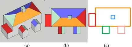
∅ (2) The combination of equation 1 and 2 are the minimum partitioning requirements, which are illustrated in Figure 2. In this paper, one sub-polygon is called a partition cell, or cell for short. An interface between two partition cells are called a partition line.
(a) (b) (c)
Figure 2. Partition requirements. The planar partition of a polygon is a sub-division of a region into non-overlapping polygons. (a) a building from perspective view; (b) top view of the building; (c) partition results of the building region according to roof layers.
Except the minimum requirements, there are several difficulties that need to be solved for achieving perfect partition results. Those questions are still open for the literature:
1. Dominant directions. Restricting partition lines to dominant directions makes the partition results beautiful, and regular. However, many buildings have no dominant directions, and some buildings has more than one dominant directions. Some directions are very close and it is very hard to decide which direction to follow.
2. Small structures. Small structures create many close candidate partition lines, resulting in lots of trivial partition cells, which increase the difficulties to merge them. Some methods in the state-of-the-art generalize the footprint and erase small structures. The generalization operation however changes footprint polygons, and is not recommended.
3. Inner building parts. A sub-building may touch the border of a footprint map, but may lie fully inside the footprint map as well. The later sub-building cannot be inferred by only considering the footprint map. Even if the height data is taken into consideration, careful efforts should be taken to detect inner building parts and to derive step edges.
4. Partition along wall or eave? The LoD1 and LoD2 models of buildings do have overhangs even though they can be generalized to have no overlap between layers. Footprints usually follow the walls while the acquired data follows roofs. Because the sensors look down, walls and lower roofs are not well observed. We can only relay on one of them where walls and eaves conflict. This question is actually the question that should we rely more on map or height data.
Considering the complexities of footprint map partitioning, we propose two algorithms in section 3 and section 4. The requirements defined by Equation 1 and Equation 2 are achieved as minimum conditions. We maintain footprint outlines but do not always partition along dominant directions.
3. METHOD1: PARTITIONING BY ROOF CONTOURS
In this section we introduce a partitioning method based on contours of roof layers. This is done by decomposing a building ISPRS Annals of the Photogrammetry, Remote Sensing and Spatial Information Sciences, Volume III-3, 2016
into layers at different height, deriving contours for each layer, and snapping those contours to footprint maps. This method relies more on height data than footprint maps.
Roof layers are derived by a component analysis of an input point cloud. The input lidar points are segmented into planar patches by a segmentation algorithm (Vosselman, 2012), and only the points on roof segments are kept by picking segments whose slop is smaller than 75°. This operation is to filter out wall points. The Triangulated Irregular Network (TIN) of the points is constructed and its long edges which exceed a certain length are deleted, afterwards the connected TIN nodes are grouped into components, each one presents a roof layers. The length criteria is determined by detail level and quality requirements. In the experiments, 2m are taken as the threshold.
The contour of a roof layer is derived by the 2D α-shape algorithm (Edelsbrunner and Mücke, 1994) and then generalized by Douglas-Peucker algorithm (Douglas and Peucker, 1973). The points of one roof layer are projected onto the X-Y plane, and the α-shape algorithm is applied. The points may have holes inside thereby one or more inner contours will also be derived. We only keep the outer contour for each roof layer. The Douglas-Peucker algorithm is designed to simplify open polylines. The start and end points are automatically marked to be kept. A line segment is constructed with the start and end points. The furthest point from the line segment is chosen as a new node if its distance is larger than a given threshold. Thereby the polyline is partitioned into two parts. Each part is iteratively partitioned in the same way until no further simplification can be applied. In our case, however, a contour is closed. We need to choose the initial start and end nodes to start simplification. This is done by picking two nodes with largest curvatures. The contour is accordingly divided into two parts, each one is simplified by the Douglas-Peucker algorithm. The points with largest curvature may not be the ideal result, therefore the initial start and end nodes are re-checked. The start or end node will be removed if it is not far enough to the line segment that is formed by its two neighbouring nodes. Figure 3 illustrates the polygon simplification algorithm.
(a) (b)
(d) (c)
Figure 3. Polygon simplification by modified Douglas-Peucker algorithm. (a) The input polygon; (b) The initial start and end nodes with maximum curvatures; (c) Simplified polygon after first round; (d) Final simplified polygon.
The regions defined by the layer contours may have overlaps and gaps in between. The conflicts are solved by snapping contours. The contour snapping is done in a way similar to Ledoux et al. (2012). Figure 4 illustrates the snapping algorithm of layer contours. By taking the footprint polygon and roof layer contours as constraints, a Delaunay Triangulation is constructed by the Constrained Delaunay Triangulation (CDT) algorithm (Chew,
1989), see Figure 4 (b). Each triangulation facet is one region cell. A region growing algorithm tags all the cells of the building regions uniquely. Each cells is ensured to only belonging to one roof layer, see Figure 4 (c). Because the input point cloud is discrete and points are not always on the footprint map, the simplified contours have small gaps with the footprint map in most situations. In order to avoid trivial triangle facets in the TIN, the roof layer contours are refined before constructing the CDT. The contour nodes are snapped to nearby nodes or line segment of the footprint polygon.
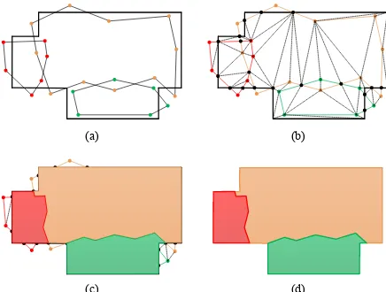
(a) (b)
(c) (d)
Figure 4. Snapping of roof layer contours. (a) The footprint map and the roof layer contours (with coloured nodes); (b) The derived Constrained Delaunay Triangulations; (c) The tagged roof regions; (d) The output of snapped contours.
The region growing algorithm guarantees the derived roof regions are continuous and gap-free. Meanwhile, it applies two growing rules: 1) The overlapped cells are set to the highest roof layer; 2) The empty cells are set to the lowest roof layer. The two rules are based on the observation that the top roof facets have higher probability to be well observed than bottom ones. Therefore the overlapped cells belong to the good data, which is the higher roof region. And the empty cells come from occlusions, therefore are set to the lost layer. On contrary to the typical polygon snapping methods, which is processed line by line, this one is done globally. It effectively guarantees the validity of resulting polygons.
4. METHOD2: PARTITIONING BY STEP EDGES
In this section, we introduce the second footprint map partitioning method by combining step edges with footprint maps. The footprint map often reveals building structures. By extending the footprint lines that cross concave corners, an initial partition will be created. Detected step edges are integrated for finer partitions. Figure 5 illustrates the pipeline of the partition algorithm.
Roof layers are detected by the component analysis algorithm introduced in Section 3. Step edges are detected from the boundaries points between each pair of adjacent roof layers. The lidar points that connect the two roof layers are identified as boundary points. And the Hough Transform algorithm is taken to detect step edges by fitting lines to the boundary points. In order to snap the partition lines to building directions, the dominant directions of a building are derived and used as constraints in the Hough Transform.
(a) (b)
(c) (d)
Figure 5. Footprint map decomposition by combining footprint map and step edges. (a) Footprint map; (b) Lidar points (coloured in height) with step edges; (c) Partition lines (in red) from footprint map with step edges; (d) Partition result.
The step edges are combined with footprint maps for finer partition. By extending footprint lines that intersect at concave corners a building ground plan can be segmented into regions. In order to avoid trivial partitions, the step edges are firstly aligned with footprint maps and their extensions, if they are close enough.
The alignment includes snapping the step edges onto footprint lines if they are close and parallel, otherwise snapping them onto footprint corners if close to them. The distance threshold is 0.5m, and angle threshold is 15°. Finer partitions are achieved by extending step lines to intersect with partition cells. The partition cells are merged according to layers of lidar points. The adjacent partition cells are merged if they are covered by a same roof layer. A partition cell may have lidar points from more than one roof layer. In this case, the cell will tagged to the roof layer with largest number of lidar points in the winner-take-all strategy.
5. EXPERIMENTS
In this section we experimentally test the improvements of partition quality by applying the two partitioning methods. Airborne lidar data and footprint maps are combined for the partitioning. The lidar data is acquired by airborne lidar systems with an average point density of 20 points/m2. Two 2D footprint data sets are tested. The first one is a large scale base map with a scale of approximately 1:500 (called MAP1). The second one is an object oriented topographic dataset with scale 1:10,000 (called MAP2). The reference data is created by manual operation with an interactive tool. Operators create partition lines along jump edges by visually checking the lidar points.
In order to evaluate the partition results, the test data are overlapped with reference data. An overlapping part is considered to be correct if it is the biggest part of the belonging polygons. For example, see Figure 7, the reference data and test data have four overlapping parts. Cell a of test data overlaps with both cell 1 and cell 2 of reference data, resulting in cell 1a, and
cell 2a. Because cell 1a has larger area than cell 2a, cell 1a is
considered to be the correct partition, and cell 2a is wrong. The
partition accuracy is defined as the ratio of area of all correct partitions with the total area of input maps.
(1a) (1b) (1c)
(2a) (2b) (2c)
Figure 6. Map partition results. Row (1) Footprint map of MAP1 and partition results; Row (2) Footprint map of MAP2 and partition results; Colum (a) Footprint maps; Colum (b) Partition results by Method1; Colum (c) Partition results by Method2.
Figure 6 shows two footprint maps and partition results by the two proposed methods. Row (1) presents footprint map of MAP1 and partition results. Row (2) presents footprint map of MAP2 and partition results. Colum (a) presents footprint maps; Colum (b) presents partition results by Method1. Colum (c) presents partition results by Method2. The partition accuracies are 89%, 96%, 91% and 90% for 1b, 1c, 2b, and 2c, respectively. The
second partitioning method creates better results on MAP1 footprint maps. While the partition accuracies have no big difference on MAP2 footprint maps.
1 2
a b
2a 2b
1a 1b
(a) (b) (c) Figure 7. Evaluation of partition. (a) Reference data; (b) Test data; (c) Comparison.
The zoom in views in Figure 8show partition results of three buildings. Partitioning method1 can identify small structures and inner structures. While partitioning method2 forces partition lines to follow building dominant directions and footprint corners. Another large difference between the two methods is the area with no data or with data from several roof layers. The conflicting parts are classified to the highest roof layer by method1, but are classified to lowest roof layer by method2. The partitioned map
can be used to reconstruct building LoD1 and LoD2 model. The reconstructed 3D models are illustrated in Figure 9, showing that the partition accuracy are good enough for the tasks of 3D modelling. Method1 is applied for the partitioning for Figure 9.
6. CONCLUSIONS
In this paper, we proposed two footprint map partition algorithm and evaluated their effects. The partition algorithms decompose a footprint map into parts, each presents an independent building part. The two proposed algorithm both apply airborne lidar data and footprint maps. The first one is more dependent on lidar data and the second one more dependent on footprint maps.
Experiments show both partition algorithms achieve up to 90% for 1:500 footprint maps and 1:10000 footprint map. In one test area the partition accuracy even reaches 96%. The partition results provide well defined polygons for detailed LoD1 modelling and LoD2 modelling. Method 1 is able to partition small roof layers, and to work in the noisy parts. Method 2 snaps partition line to dominant directions and corners, thereby the results are regular and well aligned with footprint map.
The future work is to combine the advantages of the two methods. The partitioning should work well for all situations, even for the situations where height data is noisy. Meanwhile the partitions should snap to dominant directions and footprint corners, if those constraints can be met. Lidar points in recent years are still expensive to acquire. The photogrammetric points are a cheap alternative and will also be used to decompose footprint maps and to reconstruct 3D models in the following work.
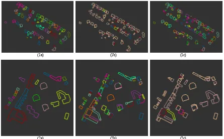
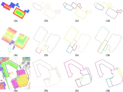
(1a) (1b) (1c) (1d)
(2a) (2b) (2c) (2d)
(3a) (3b) (3c) (3d)
Figure 8. Map partition results. Row (1) Building 1 from MAP1; Row (2) Building 2 from MAP1; Row (3) Building 3 from MAP2; Colum (a) lidar points; Colum (b) Reference partitions; Colum (c) Partition results by Method 1; Colum (d) Partition results by Method 2.
7. ACKNOWLEDGMENT
This work is part of the research programme 3D4EM, which is supported by the Dutch Technology Foundation STW, which is part of the Netherlands Organisation for Scientific Research (NWO), and which is partly funded by the Ministry of Economic Affairs.
REFERENCES
Chew, L.P., 1989. Constrained delaunay triangulations. Algorithmica, 4(1-4): 97-108.
Commandeur, T.J.F., 2012. Footprint decomposition combined with point cloud segmentation for producing valid 3D models, Technology University of Delft, Delft, The Netherlands.
Douglas, D.H. and Peucker, T.K., 1973. Algorithms for the reduction of the number of points required to represent a digitized line or its caricature. Cartographica: The (2a) (2b)
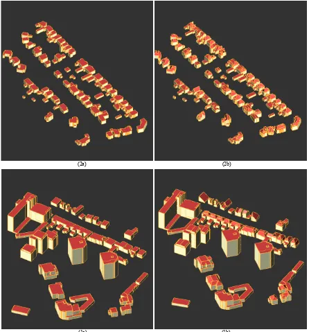
(1a) (1b)
Figure 9. 3D building modelling from partitioned footprints by method1. (1a) Detailed LoD1 models from MAP1; (1b) LoD2 models from MAP1; (2a) Detailed LoD1 models from MAP2; (2b) LoD2 models from MAP2.
International Journal for Geographic Information and Geovisualization, 10(2): 112-122.
Edelsbrunner, H. and Mücke, E.P., 1994. Three-dimensional alpha shapes. ACM Transactions on Graphics (TOG), 13(1): 43-72.
Haala, N., Becker, S. and Kada, M., 2006. Cell decomposition for the generation of building models at multiple scales, Symposium Photogrammetric Computer Vision. The International Archive of Photogrammetry, Remote Sensing and Spatial Information Sciences, pp. 19-24.
Haala, N. and Kada, M., 2010. An update on automatic 3D building reconstruction. ISPRS Journal of Photogrammetry and Remote Sensing, 65(6): 570-580. Kada, M., 2009. The 3D Berlin Project, Photogrammetric week. Wichmann Verlag, Heidelberg, Fritsch, D. (Ed.), pp. 331-340.
Kada, M. and McKinley, L., 2009. 3D building reconstruction from LiDAR based on a cell decomposition approach. International Archives of Photogrammetry, Remote Sensing and Spatial Information Sciences, 38(Part 3/W4): 47-52.
Kolbe, T., Nagel, C. and Stadler, A., 2009. CityGML—OGC standard for photogrammetry, In: Fritsch, D. (Ed.), Photogrammetric Week 2009, Wichmann Verlag, Heidelberg, pp. 265–277.
Lafarge, F., Descombes, X., Zerubia, J. and Pierrot-Deseilligny, M., 2008. Automatic building extraction from DEMs using an object approach and application to the 3D-city modeling. ISPRS Journal of photogrammetry and remote sensing, 63(3): 365-381.
Lafarge, F. and Mallet, C., 2012. Creating Large-Scale City Models from 3D-Point Clouds: A Robust Approach with Hybrid Representation. International Journal of Computer Vision: 1-17.
Ledoux, H., Arroyo Ohori, K. and Meijers, M. (2012). Automatically repairing invalid polygons with a constrained triangulation. Proceedings of the AGILE 2012 International Conference, Avignon, France, Agile, 13-18.
Oude Elberink, S., Stoter, J., Ledoux, H. and Commandeur, T., 2013. Generation and Dissemination of a National Virtual 3D City and Landscape Model for the Netherlands. Photogrammetric Engineering & Remote Sensing, 79(2): 147-158(12).
Oude Elberink, S. and Vosselman, G., 2009. Building reconstruction by target based graph matching on incomplete laser data: Analysis and limitations. Sensors, 9(8): 6101-6118.
Sohn, G., Huang, X. and Tao, V., 2008. Using a binary space partitioning tree for reconstructing polyhedral building models from airborne lidar data. Photogrammetric Engineering and Remote Sensing, 74(11): 1425-1440. Suveg, I. and Vosselman, G., 2004. Reconstruction of 3D
building models from aerial images and maps. ISPRS Journal of Photogrammetry and Remote Sensing, 58(3–4): 202-224.
Thiele, A., Hinz, S., Cadario, E. and Lacoste, H. (2010). Fusion of InSAR and GIS data for 3D building reconstruction and change detection. Proceedings of ‘Fringe 2009 Workshop’, Frascati, Italy, ESA SP-677, http://earth.eo.esa.int/workshops/fringe09/.
Vallet, B., Pierrot-Deseilligny, M., Boldo, D. and Brédif, M., 2011. Building footprint database improvement for 3D reconstruction: A split and merge approach and its evaluation. ISPRS Journal of Photogrammetry and Remote Sensing, 66(5): 732-742.
Van Winden, K., 2012. Automatically Constructing the Third Dimension of IMGeo, Utrecht University, Utrecht, The Netherlands.
Vosselman, G., 2012. Automated planimetric quality control in high accuracy airborne laser scanning surveys. ISPRS Journal of photogrammetry and remote sensing, 74: 90-100.
Vosselman, G. and Suveg, I., 2001. Map based building reconstruction from laser data and images. Automatic Extraction of Man-Made Objects from Aerial and Space Images (III). A.A. Balkema Publishers, Centro Stefano Franscini, Monte Verita,` Ascona.
Xiong, B., Oude Elberink, S. and Vosselman, G., 2014a. Building modeling from noisy photogrammetric point clouds. ISPRS Ann. Photogramm. Remote Sens. Spatial Inf. Sci., II-3: 197-204.
Xiong, B., Oude Elberink, S. and Vosselman, G., 2014b. A graph edit dictionary for correcting errors in roof topology graphs reconstructed from point clouds. ISPRS Journal of Photogrammetry and Remote Sensing, 93: 227-242. ISPRS Annals of the Photogrammetry, Remote Sensing and Spatial Information Sciences, Volume III-3, 2016