Comparing the value of Southern Oscillation Index-based climate
forecast methods for Canadian and US wheat producers
Harvey S.J. Hill (Graduate Research Assistant)
a,
Jaehong Park (Graduate Research Assistant)
a, James W. Mjelde (Professor)
a,∗,
Wesley Rosenthal (Assistant Professor)
b, H. Alan Love (Associate Professor)
a,
Stephen W. Fuller (Professor)
aaDepartment of Agricultural Economics, Texas A&M University, College Station TX 77843-2124, USA bBlackland Research Center of the Texas Agricultural Experiment Station in Temple, TX, USA
Received 9 April 1999; received in revised form 22 October 1999; accepted 31 October 1999
Abstract
Southern Oscillation Index (SOI) based forecasting methods are compared to determine which method is more valuable to Canadian and US wheat producers. Using decision theory approach to valuing information, the more commonly used three-phase method of El Niño, La Niña, and other is compared to a five-phase system. Because of differences in growing season and yearly SOI classification schemes, two different three-phase methods are used. The five-phase system is based on the level and rate of change of the SOI over a 2 month period. Phases are consistently negative, consistently positive, rapidly falling, rapidly rising, and near zero. As expected, results vary by the method used. Winter wheat producers in Illinois place no value on either of the SOI-based forecasting systems. Producers at seven of the 13 sites prefer the five-phase method over either of the three-phase method (spring wheat producers in Manitoba, Alberta, North Dakota and South Dakota, along with winter wheat producers in Oklahoma, Texas, and Washington). The value of the five-phase approach is up to 70 times more valuable than the three-phase approach. Producers growing spring wheat in Saskatchewan and Montana, along with winter wheat producers in Ohio and Kansas value the three-phase approach more than the five-phase. In this case, the value of the three-phase system is up to two times more valuable than the five-phase system. Depending on expected price and region, the values of the SOI-based forecasts range from 0 to 22% of the value of perfect forecasts. In both absolute and percentage of perfect forecasts, producers in Oklahoma, Texas, Manitoba, Saskatchewan, and South Dakota value either system more than producers in the remaining regions. Economic value and distributional aspects of the value of climate forecasts have implications for producers, policy makers, and meteorologists. Finally, the results clearly suggest all producers will not prefer one forecast type. Forecasts need to be tailored to specific regions. ©2000 Elsevier Science B.V. All rights reserved.
Keywords:El Niño/Southern Oscillation; Value of information; Wheat
∗Corresponding author. Tel.:+1-409-845-2116; fax:+1-409-862-1563.
E-mail address:[email protected] (J.W. Mjelde).
1. Introduction
El Niño/Southern Oscillation (ENSO) events have recently received considerable attention. Various stud-ies have shown ENSO events in the tropical Pacific
are teleconnected (linked) to seasonal climate vari-ations in other parts of the world (Bjerknes, 1969; Ropelewski and Halpert, 1986, 1987, 1989; Kiladis and Diaz, 1989). Economic-based studies (Marshall et al., 1996; Mjelde et al., 1997; Hill et al., 1998) have shown these events to have value to decision-makers because of their ability to forecast climate conditions. Classifying ENSO events and the terminology asso-ciated with the ENSO phenomenon, however, are not standardized. The objective of this study is to com-pare different ENSO classification methods to deter-mine which provides greater value to Canadian and US wheat (Triticum aestivumL.) producers.
Current methods to classify ENSO events rely on sea surface temperature anomalies, sea surface air pressure differences across the Pacific, or some combination of these and other weather parameters. Methods using the Southern Oscillation Index (SOI) rely on sea surface air pressure differences. There are at least two SOI-based climate forecasting meth-ods. The most commonly used method classifies SOI events into three phases (3P): low SOI (El Niño), other, and high SOI (La Niña) (Climate Prediction Center, 1998). Within the three-phase method, two different classification schemes are used in this study. A second method classifies SOI events into five phases (5P): consistently negative, consistently pos-itive, rapidly falling, rapidly rising, and consistently zero (Stone and Auliciems, 1992). Only these two SOI-based forecast methods, along with perfect fore-casts, are considered because sea surface temperature data are not available for a sufficient period to provide meaningful comparisons. This study is the first formal attempt to compare the economic value of different SOI-based forecast methods.
2. Methodology
Currently, few wheat producers are integrating SOI-based climate forecasts into their management practices because many are unaware of this informa-tion or lack the knowledge to use this informainforma-tion (Nicholls, 1999). Consequently, data containing pro-ducers’ responses to improved climate forecasts are not available. One method to overcome data limita-tions is to use biophysical simulation models. Such a simulation model in combination with decision theory
is used to identify the value of the 3P, 5P, and perfect forecasting methods.
2.1. Crop growth simulation model
The crop growth model used in this study is the CERES-wheat model (Godwin et al., 1990). The CERES-wheat model is selected because of its de-tail and inclusiveness regarding wheat growth and development. This model is a process-oriented, man-agement level model of wheat crop growth and devel-opment that simulates soil water balance and nitrogen balance associated with plant growth. The model requires daily weather (maximum and minimum tem-perature and precipitation), soil, and variety-specific genetic characteristics. CERES-wheat has been veri-fied and used to assess different management strate-gies in various locations (Savin et al., 1995; Pecetti and Hollington, 1997).
2.2. Site descriptions and data
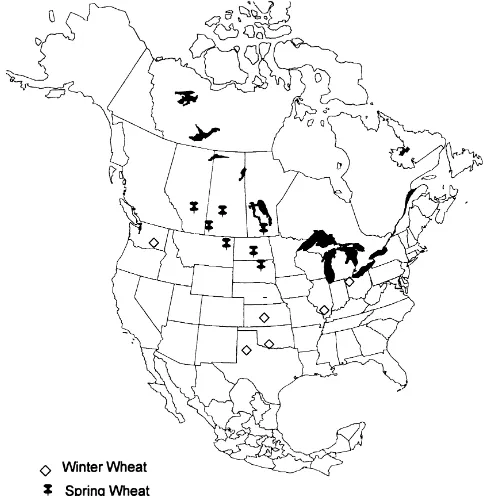
Six sites within the major winter wheat producing regions in the US are modeled, whereas seven sites are modeled to represent major Canadian and US spring wheat-growing regions. Approximate locations of the sites are given in Fig. 1. Descriptions of the sites are presented in Table 1. The dominant wheat class grown in each region is modeled. Canadian western red spring wheat is the only wheat class modeled in Canada. Hard red spring wheat is modeled in North and South Dakota and Montana. Hard red winter wheat is modeled in Kansas, Oklahoma, and Texas. Soft red winter wheat is modeled in Illinois and Ohio. Soft white winter wheat is modeled in Washington. Rep-resentative soil characteristics appropriate for wheat growing are identified in Canada using the Soil Land-scapes of Canada maps (Agriculture Canada, 1986a, b, 1991) and in the US using the Map Unit Use File (MUUF) (Baumer et al., 1984).
Fig. 1. Locations of spring and winter wheat sites.
Table 1
Site and parameter description for modeled wheat sites
Site name Longitude/latitude (north/west) Soil type Wheat class Julian planting datesa Seed rate (seeds/ha)b
US winter wheat
Illinois 39–89 Silt loam Soft red 250, 265, 280 3,500,000
Kansas 38–98 Sandy loam Hard red 240, 255, 270 3,500,000
Ohio 41–84 Silt loam Soft red 250, 265, 280 4,750,000
Oklahoma 36–98 Silt clay Hard red 240, 255, 270 3,500,000
Texas 33–99 Silt clay Hard red 240, 255, 270 1,875,000
Washington 48–118 Silt loam Soft white 240, 255, 270 2,500,000
US spring wheatc
Montana 48–110 Silt loam Hard red 95, 110, 115 3,000,000
North Dakota 48–97 Silt loam Hard red 95, 110, 115 4,750,000
South Dakota 45–98 Silt loam Hard Red 95, 110, 115 4,750,000
Canada spring wheatd
Carmen, Man. 49–98 Clay loam Western red 120, 135, 150 2,750,000
Aneroid, Sask. 49–108 Clay loam Western red 120, 135, 150 1,875,000 Watson, Sask. 52–106 Clay loam Western red 125, 140, 155 2,750,000 Vermilion, Alta. 52–111 Clay loam Western red 120, 135, 150 2,750,000
aDay of year in Julian days. bSeeds per hectare. cHard red spring.
are from USDA-Economic Research Service (1996) regional farm budgets for the years 1989–1995. Costs are adjusted to 1997 prices assuming an annual 3% inflation rate. The price of nitrogen incorporated into the model is the mean price for the period 1989–1995 (U.S.D.A.-N.A.S.S., 1996). Five wheat prices (varies slightly by site because of regional differences) rep-resenting the historic range of wheat prices for each wheat class are used.
Weather data are from Environment Canada (1997) and the US Historical Climatological Network (East-erling et al., 1998; Kaiser, 1998). Solar radiation is ap-proximated using a solar radiation generator (Richard-son and Wright, 1984). Missing information regarding precipitation and/or temperature data is approximated by incorporating data from a nearby location or if no location is available by use of a random weather gener-ator, WGEN (Richardson and Wright, 1984). Because winter wheat is planted in the fall and harvested the next year, 86 years (1910–1985) of weather data are used to represent 85 cropping years.
Two different procedures to classify the weather years are used for the 3P method. The first method uses the classification of SOI events by the Climate Prediction Center (CPC) (1998). Because information that may not be available at planting time for winter wheat is used in making these classifications, a second method is also used to classify the 3P events. The CPC yearly classification, which extends roughly from Oc-tober of yeart through September of yeart+1, may use information on ENSO that is not available until af-ter the assumed October planting dates. In classifying the years and yields in this study, the CPC classifica-tion of yeart is used to classify yeart+1 yields. To clarify, consider 1920. The classification of 1920’s is used to impact 1921’s yields (planting occurs in the fall 1920 but harvest occurs in 1921). Thus, the CPC’s October through September classification is consistent with the winter wheat growing season. In the second method, the years are classified based on the average of the July, August, and September standardized SOI. If the average value is 0.6 or above is classified as La Niña year, whereas a value of−0.6 is classified as an El Niño event. Years with an average value between −0.6 and 0.6 are classified as other years.
For spring wheat producers, two similar tion procedures are used. First, the CPC’s classifica-tion is used. As with winter wheat the classificaclassifica-tion is
lagged in terms of its impact on spring wheat yields. The lagged procedure is used because the classification is based primarily on the winter SOI values. ENSO’s main impact on weather is in the October–April/May time frame. The second method uses the−0.6 and 0.6 values to classify years using the average standardized SOI value for February, March, and April. Under this method, the producer uses updated information on the SOI value in decision making.
The years are divided into five phases according to the 5P-classification scheme developed by Stone and Auliciems (1992). Because winter wheat is planted in the fall, classification of the SOI event is based on the September classification. Missing phase classifi-cations for winter wheat are obtained by interpolating the first available monthly SOI number before and af-ter September. For spring wheat, April is selected as the basis of the SOI phase.
Classification of the years in this study is presented in Appendix A. Although the classifications are sim-ilar, there are differences between the classification. These differences give rise to different expected val-ues of the SOI-based forecasts.
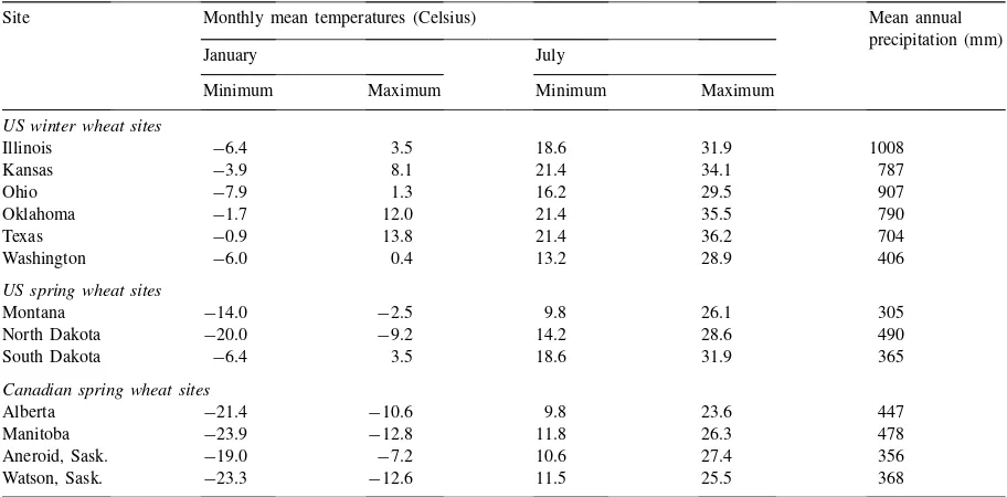
Maximum and minimum temperatures for January and July, along with mean annual precipitation, are presented in Table 2. A range of environmental condi-tions is modeled across the different sites. For exam-ple, mean annual precipitation ranges from 300 mm at the Montana site to 1008 mm at the Illinois site.
2.3. Economic decision model
Table 2
Site climate characteristics for the years 1910–1994a
Site Monthly mean temperatures (Celsius) Mean annual
precipitation (mm)
January July
Minimum Maximum Minimum Maximum
US winter wheat sites
Illinois −6.4 3.5 18.6 31.9 1008
Kansas −3.9 8.1 21.4 34.1 787
Ohio −7.9 1.3 16.2 29.5 907
Oklahoma −1.7 12.0 21.4 35.5 790
Texas −0.9 13.8 21.4 36.2 704
Washington −6.0 0.4 13.2 28.9 406
US spring wheat sites
Montana −14.0 −2.5 9.8 26.1 305
North Dakota −20.0 −9.2 14.2 28.6 490
South Dakota −6.4 3.5 18.6 31.9 365
Canadian spring wheat sites
Alberta −21.4 −10.6 9.8 23.6 447
Manitoba −23.9 −12.8 11.8 26.3 478
Aneroid, Sask. −19.0 −7.2 10.6 27.4 356
Watson, Sask. −23.3 −12.6 11.5 25.5 368
aSource: Easterling et al. (1998) and Environment Canada (1997).
whereπh,i (p) is the maximum expected net returns
per hectare (ha) for the climatological distribution of climate given pricep,Tis the number of years (85),pis expected price per kilogram ($/kg),yijis yield (kg/ha)
associated with siteiand yearj,nis applied nitrogen in kg/ha,dis planting date,r1is nitrogen cost in $/kg,
r2 is harvest costs in $/kg, and vci is other variable
costs in $/ha. Eight different nitrogen levels (15, 30, 45, 60, 75, 90, 115, and 120 kg/ha) are modeled for each site. Three different planting dates, representing a range of dates are modeled per site (see Table 1). Planting dates vary by site because of environmental conditions. Letxi* represent the optimal combination
of planting date and applied nitrogen associated with use of the decision maker’s prior knowledge. Note, that for each site only one combination (one planting date and one applied nitrogen level) is obtained when the producer is using only prior knowledge.
The model used to obtain the expected returns for each forecasted phase is:
πk,i(p)=max n,d
1 Tk
Tk X
j=1
p yij(n, d)
−r1n−r2yij(n, d)−vci
(2)
whereπk,i (p) is the maximum expected net returns
per ha for forecasted eventkgiven pricep,Tk is the
number of years represented by each climate forecast.
Tk corresponds to the subset of years that are
associ-ated with the specific climate phase forecasted. In the 3P method,kequals 1, 2, or 3, whereask=1,. . ., 5 in the 5P method. When perfect forecasts are valued,Tk
equals 1, because with a perfect forecast each years’ climatic variability is known. Let zk,i* represent the
optimal input combination for the climate conditions following phase kfor site i. Note, an optimal input combination is determined by phase for each site. Ei-ther three or five different input combinations are pos-sible depending on forecast method.
Optimal expected net returns by phase are given by Eq. (2). To obtain the expected net returns for a given method, net returns for a phase are weighted by the probability of the phase occurring. Mathematically, the expected net returns are
πi(p)= M
X
m=1
wmπm,i(p) (3)
wherewmis the probability of phasemoccurring and
modeled. The value of the forecast information is dif-ference between the expected net returns with and without SOI-based forecasts
Vi(p)=πh,i(p)−πi(p) (4)
where,Vi (p) is the expected value (additional net
re-turns) of the forecasting system for siteigiven price
p. Obtaining the value of the forecast in this man-ner is consistent with previous value of information studies (Hilton, 1981; Mjelde et al., 1997; Hill et al., 1998). For the information system to have value, the SOI-based forecasts must alter the optimal input com-bination relative to the prior knowledge case for at least one of the phases. That is, for either SOI-based method to have value,zk,i* cannot equalxi* for allk.
Changes in input usage effect returns through wheat yield changes (caused by adjustments in applied nitro-gen level and planting date) and costs through changes in applied nitrogen level. Changes in returns and costs are reflected in the value of the forecasts. This process is repeated for each of the five price levels.
3. Results and discussion
The expected values of the 3P, 5P, and perfect fore-casts for spring and winter wheat producers vary by site and price (Tables 3 and 4). In some locations, the SOI-based information is of no greater value than cli-matological information. As expected, at all sites the value of perfect information is greater than the value of either the 3P or 5P forecast method. Although changes in inputs usage caused by the use of ENSO-based fore-casts are not presented because of space considera-tions, the value of the forecasts (additional net returns) results from the changes in input use.
3.1. Winter wheat sites
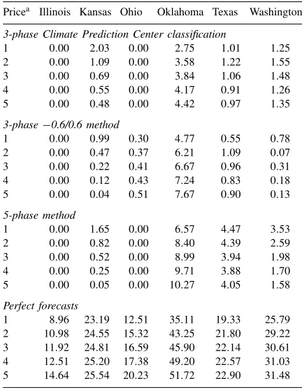
Use of either 3P method in Illinois provides no value to the producers (Table 3). At the Ohio site, the CPC’s classification has no value and the −0.6/0.6 method has little value. For the remaining four sites, additional net returns range from US$ 0.55/ha in Texas to US$ 4.77/ha in Oklahoma at the lowest wheat price. At the highest wheat price, additional net returns range from US$ 0.04/ha in Kansas to US$ 7.67/ha in Okla-homa. Differences between sites are also noted in the
Table 3
Value to US hard winter wheat producers (US$/ha) of SOI-based climate forecasts
Pricea Illinois Kansas Ohio Oklahoma Texas Washington
3-phase Climate Prediction Center classification
1 0.00 2.03 0.00 2.75 1.01 1.25
aBecause of differences in regional prices, the analysis uses
dif-ferent prices for each region. For Kansas, Oklahoma, and Texas the five prices are US$ 91.97, 117.60, 125.84, 135.99, and 143.73/kg. For Illinois and Ohio the prices are US$ 89.43, 110.49, 120.05, 125.95, and 147.03/kg and for Washington the prices are US$ 97.30, 117.60, 132.50, 140.30, and 148.00/kg.
pattern of values over the range of prices. In Kansas, forecast value decreases as the wheat price increases, whereas in Oklahoma an opposite pattern is noted. For Texas and Washington, the forecast value increases as wheat price increases at the lower prices, whereas at the higher prices the forecast value declines as price increases. This result is consistent with previous find-ings on the determinants of information value. Hilton showed there is no monotonic relationship between the determinants of information value (in this case wheat price) and the value of information.
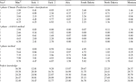
Table 4
Value to Canadian and US hard red spring wheat producers (US$/ha) of SOI-based climate forecasts
Pricea Man.b Sask. 1 Sask. 2 Alta. South Dakota North Dakota Montana
3-phase Climate Prediction Center classification
1 1.99 0.41 0.95 0.37 2.68 0.59 1.46
2 2.47 0.95 2.30 0.37 2.37 0.71 1.17
3 3.84 2.13 4.72 0.55 2.24 0.93 0.94
4 4.23 4.45 5.77 0.87 2.19 1.09 0.88
5 6.15 6.23 6.92 1.21 2.23 1.36 0.82
3-phase−0.6/0.6 method
1 1.94 0.03 0.00 0.00 0.07 0.11 1.34
2 2.66 0.14 1.02 0.00 0.00 0.00 0.90
3 3.69 0.61 1.68 0.07 0.00 0.00 0.80
4 4.63 2.00 2.20 0.00 0.00 0.00 0.88
5 6.38 2.41 2.70 0.00 0.13 0.00 1.06
5-phase method
1 5.02 0.00 0.59 0.64 4.95 1.19 0.91
2 5.64 0.84 2.14 0.97 4.72 1.02 0.25
3 7.35 2.13 3.96 0.71 5.08 1.14 0.25
4 7.99 3.81 4.93 0.94 5.44 1.42 0.43
5 9.78 4.47 6.07 1.58 5.82 1.78 0.61
Perfect knowledge
1 16.38 12.01 9.20 13.87 29.67 22.25 26.37
2 19.38 20.19 16.76 16.99 31.75 24.41 28.73
3 24.28 24.94 22.07 19.30 33.66 26.26 30.79
4 26.47 30.81 28.09 20.90 35.13 27.69 32.36
5 32.49 34.47 32.77 23.80 36.78 29.21 34.09
aBecause of differences in regional prices, the analysis uses different prices for each region. Prices for the US sites are US$ 111.25,
131.88, 147.71, 159.17, and 171.46/kg. For Alberta sites the prices are US$ 56.43, 77.03, 96.81, 115.42, and 132.09/kg, for Saskatchewan the prices are US$ 54.12, 66.48, 86.05, 109.00, and 130.71/kg, and for Manitoba US$ 61.32, 71.50, 87.90, 96.04, and 116.69/kg.
bAbbreviations are Carmen, Manitoba, Aneroid, Saskatchewan, Watson, Saskatchewan, Vermillion, Alberta.
returns almost double between the CPC and−0.6/0.6 scheme. This result is unexpected, because the CPC uses information beyond October (planting time) to classify the years. It was expected such additional information would provide increase value. By using additional information, however, the classification maybe ignoring conditions early in the growing sea-son that may have a greater impact on yields than later conditions. At Kansas, Texas, and Washington sites, the CPC method provides higher value.
Very similar patterns are observed with the 5P method. Illinois and Ohio producers obtain no value from using the 5P method. At the four remaining sites, additional net returns range from US$ 1.65/ha in Kansas to US$ 6.57/ha in Oklahoma at the low-est wheat price. At the highlow-est price, additional net returns range from US$ 0.05/ha in Kansas to US$ 10.27/ha in Oklahoma. The value of the forecast
across price follows patterns similar to those observed for the 3P method, except for Washington. At the Washington site, the value of the forecast decreases as wheat price increases. Depending on the 3P method selected, the site, and price, the value associated with the 5P method ranges from 0.1 to 12.1 times the value of the 3P forecasts (ignoring sites and prices with an expected value of zero for the 3P and/or 5P methods). Differences in the value of the forecasts are partially caused by the climatic variability experienced at each site and the strength of the association between climatic variability and the Southern Oscillation.
pattern not consistent with the SOI-based forecast methods for some sites.
The value of SOI-based forecasts is not uniform across regions. Development and use of SOI-based forecasts will potentially benefit some producers more than others. Income distributional questions these re-sults raise, however, are beyond the scope of this study. These distributional issues need to be addressed in a larger societal context. The value of the 3P and 5P methods within a region are not equal except for Illi-nois producers. With the exceptions of the Ohio site and the Kansas site at the lowest two prices, the 5P method yields a higher value than either 3P method.
In Washington, Kansas, and Texas the 3P-CPC method captures 5, 9, and 5% of the value of perfect forecasts at the lowest price, whereas the −0.6/0.6 method captures 3–4%. At the highest price, the 3P-CPC and−0.6/0.6 methods capture less than 4% of the value of perfect forecasts in Kansas, Texas, and Washington. In Oklahoma, the 3P-CPC method captures approximately 8%, whereas the −0.6/0.6 method captures 14% of the value of perfect knowl-edge at both the highest and lowest price. In Illinois, no method captures any portion of the value of per-fect forecasts. The−0.6/0.6 method in Ohio captures approximately 2% of the value of perfect forecasts, whereas the CPC method captures none of the value. Except for the Midwest sites and Kansas, the 5P method captures a higher percentage of the value of perfect forecasts at all prices. Kansas producers obtain more value from the 3P-CPC method at low prices and the 5P method at higher prices. At the lowest price, the percentage of the value of perfect forecasts captured by the 5P method for Texas, Oklahoma, Washington, and Kansas are 23, 19, 14, and 7%, whereas at the highest price, these percentages are 18, 19, 5, and 0%. The comparatively high percentage of the value of perfect forecasts captured by the SOI-based methods suggests skill is present in the current SOI-based forecasts. Economic results mirror meteorological relationships between SOI events and weather pat-terns. The strongest relationships between the SOI and climate variability have been found in the South and Northwest (Ropelewski and Halpert, 1986, 1987, 1989; Kiladis and Diaz, 1989). Previous meteoro-logical findings corroborate the results of this study which shows greater value to ENSO-based forecasts in Oklahoma, Texas, and Washington. Further, in
Oklahoma, SOI-based forecasts may capture a large percentage of the perfect forecast’s value because Oklahoma lies near the boundary between two Pa-cific North American (PNA) atmospheric pressure patterns. The PNA is an important teleconnection pat-tern in the US (Wallace and Gutzler, 1981). Further, it appears there are interactions between the PNA and SOI (Nemanishen, 1998). Weaker signals have been found between ENSO and climate variability for the Midwest and Great Plains (Ropelewski and Halpert, 1986, 1987, 1989). Weather, soil types, and wheat type also effect the value of the SOI-based forecasts. Illinois and Ohio are areas with fertile soils and more advantageous rainfall patterns than other wheat growing areas. This growing environment in combi-nation with the regions’ weak SOI signal appears to reduce the value of SOI-based and perfect knowledge forecasts.
3.2. Spring wheat results
For the spring wheat sites, the relationship between 3P, 5P, and perfect forecasts is different (Table 4) than for winter wheat. The 3P-CPC method provides more valuable forecasts than the −0.6/0.6 method at all sites, except the Manitoba site where the two meth-ods have nearly identical expected values. At three sites, Alberta, South Dakota, and North Dakota, the −0.6/0.6 method has no value. For the sites showing positive value from using the 3P-CPC method at the lowest wheat price, additional net returns range from US$ 0.41/ha for the Aneroid, Saskatchewan site to US$ 2.68/ha in South Dakota. At the wheat highest price, additional net returns range from US$ 0.82/ha in Montana to US$ 6.92/ha in Watson, Saskatchewan. Further, at the Montana and South Dakota sites, the value of the forecast decreases as the producer’s expected price increases. At the remaining sites the converse is true.
clearly discernible pattern between the forecast value and the expected price level.
The value of perfect forecasts increased consistently as wheat price increases. At the lowest price, addi-tional net returns associated with perfect forecast range between US$ 9.20 and 29.67/ha. At the highest price, additional net returns range between US$ 23.80 and 36.78/ha.
The value of SOI-based climate forecasts for spring wheat production is not uniform across regions, again raising income distribution issues. All spring wheat producing sites benefit from using the 3P or 5P fore-cast methods, although for some sites, method, and prices, the benefit is small. With three exceptions, the two Saskatchewan sites and the Montana site, the 5P method provides greater value to spring wheat pro-ducers than the 3P method.
With the 3P-CPC method, the sites with positive forecast value capture at the lowest price between 3 and 12% of the value of the perfect forecast. At the highest price, the 3P-CPC method captures be-tween 2 and 19% of the value of perfect forecasts. The−0.6/0.6 method captures between 0.2 and 12% of the value of a perfect forecast at the lowest price, whereas between 0.3 and 20% is captured at the high-est price. At the lowhigh-est price, the 5P method captures 3.4–22% of the value of perfect forecasts, whereas at the highest price, the 5P forecasts capture 1.8–30% of the perfect forecast information. For spring wheat, the 5P method ranges between 0.03 and 70 times more valuable than the 3P methods (as before ignoring sites that have zero expected value).
3.3. Value comparison by phase
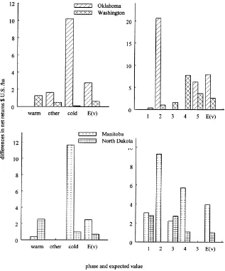
The question remains, ‘does knowledge of every phase or does knowledge of only certain phases pro-vide value to the producer?’ Oklahoma and Washing-ton sites are used to address this question for win-ter wheat, while Manitoba and North Dakota sites are used as spring wheat examples. These sites provide different answers to this question. The reader is cau-tioned that the results are site specific and generaliza-tions are difficult. Differences in expected net returns using the 5P and 3P-CPC forecast methods for the Ok-lahoma and Washington sites are presented in Fig. 2 by phase for price level two. As noted earlier, these differences in expected net returns arise from changes
in input usage. At the Oklahoma site, changes in in-put use and consequently changes in expected net re-turns occur in the other and cold phase when using the 3P-CPC method (Fig. 2), although the majority of the value arises during the cold phase. Using the 5P method, input usage changes over the prior knowl-edge strategies in Phases 2 and 5. Phase 2 is similar to the cold event in the 3P-CPC, whereas Phase 5 cor-responds somewhat to the other event in the 3P-CPC method. In contrast, decision makers in Washington alter input use in all phases when using either the 3P-CPC or 5P forecasts. Phase 4 additional net returns is small, however.
In the 3P-CPC method, the cold and warm phases provide the Manitoba and North Dakota producers with valuable information. Manitoba producers gain more from the cold phase, whereas North Dakota pro-ducers obtain more value from information concern-ing the warm phase. For the 5P method, Manitoba has additional net returns in Phases 1, 2, 3, and 4, whereas North Dakota producers’ net returns increase in Phases 1, 3, and 4.
4. Conclusions
The objective of this study is to compare differ-ent SOI-based forecast methods to determine which provides greater value to Canadian and US wheat producers. For three of the six winter wheat sites modeled (Oklahoma, Texas, and, Washington) the 5P method provides more valuable information than the 3P method. The preferred method for Kansas win-ter wheat producers depends on the price, although the differences between methods are small. Neither method provides any value at the Illinois winter wheat sites and little value to Ohio producers. Depending on price, site, and forecast method between 0 and 23% of the value of perfect forecasts are captured using the SOI-based forecasts.
For spring wheat producing sites, the 5P method provides more valuable information than the 3P method in four of the seven sites. The forecast values ranged between 0 and 30% of the value of perfect forecasts depending on the price, site, and forecast method.
Fig. 2. Differences in net returns from the use of the 5 phase and 3 phase-CPC forecasting methods by phase selected winter and spring wheat sites.
a fixed price. But more important, the results sug-gest that one type of forecast may not fit all produc-ers or regions. Forecasts need to be tailored to spe-cific regions. These conclusions have implications for the US and Canadian climate forecasting systems and decision-makers using the information. It also illus-trates the need for multi-disciplinary interaction and research between decision-makers, social scientists, and physical scientists, if improved climate forecasts are to reach their full potential.
Future research should utilize other forecasting methods besides the SOI. In the near future the
Acknowledgements
This research was partially supported by Depart-ment of Commerce, National Oceanographic and At-mospheric Administration Grant NA66GPO189.
Appendix A. Classification of the years into ENSO Phases (l9xx)
Three phase method—Climate Prediction Center
—fall and spring (lag value for crop year—see text) Warm phase (1): 11, 14, 18, 23, 25, 30, 32, 39, 41,
Three phase 60/60 method—Fall
Warm phase (1): 11, 13, 14, 18, 19, 23, 25, 26, 32,
Three phase 60/60 method—Spring
Warm phase (1): 12, 19, 21, 26, 32, 40, 41, 42, 53,
Five phase method—Fall
Phase 1 11, 25, 23, 34, 40, 41, 53, 57, 65, 72, 76,
Five phase method—Spring
Phase 1 26, 40, 41, 66, 77, 80, 81, 83, 87, 91, 92
Agriculture Canada, Soil Landscapes of Canada: Alberta, 1986a. Pub. 5242/B, Land Resource Centre, Research Branch, Ottawa. Agriculture Canada, Soil Landscapes of Canada: Manitoba, 1986b. Pub. 5237/B, Land Resource Centre, Research Branch, Ottawa. Agriculture Canada, Soil Landscapes of Canada: Saskatchewan, 1991. Pub. 5243/B, Land Resource Centre, Research Branch, Ottawa.
Alberta Agriculture, 1989–1995. Crop Production Cost and Returns — Brown Soil Zone, Lethbridge, Dryland. Economic Services, Edmonton, Alberta.
Baumer, O., Kenyon, P., Bettis, J., 1984. MUUF v2.14 User’s Manual. National Resources Conservation Service, 520 pp. Bjerknes, J., 1969. Atmospheric teleconnections from the
equatorial Pacific. Monthly Weather Rev. 97 (3), 163–172. Climate Prediction Center, 1998. El Niño (ENSO) — Previous
Warm and Cold Episode Years. National Oceanographic and Atmospheric Agency, web site http://nic.fb4.noaa.gov:80/ products/analysis monitoring/ensostuff/index.html.
Easterling, D.R., Karl, T.R., Mason, E.H., Hughes, P.Y., 1998. U.S. Historical Climatology Network Daily Temperature and Precipitation Data. ORNL/CDIAC NDP-042/R1, Carbon Dioxide Information Analysis Center, Oak Ridge National Laboratory, Oak Ridge, TN.
Godwin, D., Ritchie, J., Singh, U., Hunt, L., 1990. A User’s Guide to CERES Wheat v2.10, 2nd Edition. International Fertilizer Development Center, Muscle Shoals, AL.
Hill, H.S.J., Mjelde, J.W., Rosenthal, W., Lamb, P.J., 1998. The potential impacts of the use of Southern Oscillation information on the Texas aggregate sorghum production. J. Climate 12 (1), 519:530.
Hilton, R.W., 1981. The determinants of information value: synthesizing some general results. Manage. Sci. 27 (1), 57–64. Kaiser, D.P., 1998. Climatologist. Personal Communication. Oak
Ridge National Laboratory, Oak Ridge, TN.
Kiladis, G.N., Diaz, H.F., 1989. Global climatic anomalies associated with extremes of the Southern Oscillation. J. Climate 2 (9), 1069–1090.
Manitoba Agriculture, 1989–1995. Operating Costs Wheat. Farm Management Section, Winnipeg, Manitoba.
Marshall, G.R., Parton, K.A., Hammer, G.L., 1996. Risk attitude planting conditions and the value to a dryland wheat grower. Aust. J. Agric. Eco. 40 (3), 211–213.
Mjelde, J.W., Thompson, T.N., Hons, F.M., Cothren, J.T., Coffman, C.G., 1997. Using Southern Oscillation information for determining corn and sorghum profit-maximizing input levels in east-central Texas. J. Prod. Agric. 10 (1), 168–175. Nemanishen, W., 1998. Drought in the Palliser Triangle (A
Provisional Primer). Prairie Farm Rehabilitation Administration. Agricultural and Agri-Food Canada, Calgary, Alberta. Nicholls, N., 1999. Cognitive Illusions, Heuristics, and Climate
Predictions. Bull. Am. Meteorol. Soc. 7 (80), 1385–1397. Pecetti, L., Hollington, P.A., 1997. Applications of the
CERES-wheat simulation to Durum wheat in two diverse mediterranean environments. Eur. J. Agron. 6 (1/2), 123–139.
Richardson, C.W., Wright, D.A., 1984. WGEN: A Model for Generating Daily Weather Variables, USDA/ARS-8, 83 pp. Ropelewski, C.F., Halpert, M.S., 1986. North American
precipitation and temperature patterns associated with the El Niño/Southern Oscillation (ENSO). Monthly Weather Rev. 114 (12), 2352–2362.
Ropelewski, C.F., Halpert, M.S., 1987. Global and regional scale precipitation and temperature patterns associated with the El Niño/Southern Oscillation. Monthly Weather Rev. 115 (8), 1606–1626.
Ropelewski, C.F., Halpert, M.S., 1989. Precipitation patterns associated with the high index phase of the Southern Oscillation. J. Climate 2 (3), 268–284.
Saskatchewan Agriculture and Food, 1997. Agricultural Statistics Handbook 1996. Regina Sask, Canada.
Saskatchewan Agriculture and Food, 1996. Farm Facts 1989–1995. Regina Sask, Canada.
Savin, R., Satorre, E.H., Hall, A.J., Slafter, G.A., 1995. Assessing strategies for wheat cropping in the monsoonal climate of the pampas using the CERES-wheat simulation model. Field Crop Res. 42 (2/3), 81–91.
Stone, R.C., Auliciems, A., 1992. SOI phase relationships with rainfall in eastern Australia, Intern. J. Climatol. 12(April):625-636.
U.S.D.A.-N.A.S.S., 1996. Fertilizer and Agricultural Limestone: Prices Paid, Region, and United States. Agricultural Prices, Washington D.C., April, B-12–B-13.