Topic 6 - Schema for coverage geometry and functions

(1)

Reference number of this OGC® project document:

OGC 07-011

Version:7.0.0

Category: OpenGIS® Abstract Specification Editor: OGC

The OpenGIS® Abstract Specification

Topic 6:

Schema for coverage geometry and functions

Copyright notice

Warning

This document is an OGC Standard. It is subject to change without notice.

Document type: OpenGIS® Abstract Specification Document subtype: not applicable

(2)

(3)

iii

(4)

Foreword

This version supercedes all previous versions of OpenGIS® Abstract Specification Topic 6, including OGC document 00-106.

This document is a joint effort and is jointly published between the Open Geospatial Consortium, Inc. and ISO (the International Organization for Standardization).

ISO (the International Organization for Standardization) is a worldwide federation of national standards bodies (ISO member bodies). The work of preparing International Standards is normally carried out through ISO technical committees. Each member body interested in a subject for which a technical committee has been established has the right to be represented on that committee. International organizations, governmental and non-governmental, in liaison with ISO, also take part in the work. ISO collaborates closely with the International Electrotechnical Commission (IEC) on all matters of electrotechnical standardization.

International Standards are drafted in accordance with the rules given in the ISO/IEC Directives, Part 2.

The main task of technical committees is to prepare International Standards. Draft International Standards adopted by the technical committees are circulated to the member bodies for voting. Publication as an International Standard requires approval by at least 75 % of the member bodies casting a vote.

Attention is drawn to the possibility that some of the elements of this document may be the subject of patent rights. Neither OGC nor ISO shall not be held responsible for identifying any or all such patent rights.

(7)

vii

Introduction

Geographic phenomena fall into two broad categories — discrete and continuous. Discrete phenomena are recognizable objects that have relatively well-defined boundaries or spatial extent. Examples include buildings, streams and measurement stations. Continuous phenomena vary over space and have no specific extent. Examples include temperature, soil composition and elevation. A value or description of a continuous phenomenon is only meaningful at a particular position in space (and possibly time). Temperature, for example, takes on specific values only at defined locations, whether measured or interpolated from other locations.

These concepts are not mutually exclusive. In fact, many components of the landscape may be viewed alternatively as discrete or continuous. For example, a stream is a discrete entity, but its flow rate and water quality index vary from one position to another. Similarly, a highway can be thought of as a feature or as a collection of observations measuring accidents or traffic flow, and an agricultural field is both a spatial object and a set of measurements of crop yield through time.

Historically, geographic information has been treated in terms of two fundamental types called vector data and raster data.

―Vector data‖ deals with discrete phenomena, each of which is conceived of as a feature. The spatial characteristics of a discrete real-world phenomenon are represented by a set of one or more geometric primitives (points, curves, surfaces or solids). Other characteristics of the phenomenon are recorded as feature attributes. Usually, a single feature is associated with a single set of attribute values. ISO 19107:2003 provides a schema for describing features in terms of geometric and topological primitives.

―Raster data‖, on the other hand, deals with real-world phenomena that vary continuously over space. It contains a set of values, each associated with one of the elements in a regular array of points or cells. It is usually associated with a method for interpolating values at spatial positions between the points or within the cells. Since this data structure is not the only one that can be used to represent phenomena that vary continuously over space, this International Standard uses the term ―coverage,‖ adopted from the Abstract Specification of the Open GIS Consortium [1]_{, to refer to any data representation that assigns values directly to} spatial position. A coverage is a function from a spatial, temporal or spatiotemporal domain to an attribute range. A coverage associates a position within its domain to a record of values of defined data types.

In this International Standard, coverage is a subtype of feature. A coverage is a feature that has multiple values for each attribute type, where each direct position within the geometric representation of the feature has a single value for each attribute type.

Just as the concepts of discrete and continuous phenomena are not mutually exclusive, their representations as discrete features or coverages are not mutually exclusive. The same phenomenon may be represented as either a discrete feature or a coverage. A city may be viewed as a discrete feature that returns a single value for each attribute, such as its name, area and total population. The city feature may also be represented as a coverage that returns values such as population density, land value or air quality index for each position in the city.

(8)

Geographic information

—

Schema for coverage geometry and

functions

1 Scope

This International Standard defines a conceptual schema for the spatial characteristics of coverages. Coverages support mapping from a spatial, temporal or spatiotemporal domain to feature attribute values where feature attribute types are common to all geographic positions within the domain. A coverage domain consists of a collection of direct positions in a coordinate space that may be defined in terms of up to three spatial dimensions as well as a temporal dimension. Examples of coverages include rasters, triangulated irregular networks, point coverages and polygon coverages. Coverages are the prevailing data structures in a number of application areas, such as remote sensing, meteorology and mapping of bathymetry, elevation, soil and vegetation. This International Standard defines the relationship between the domain of a coverage and an associated attribute range. The characteristics of the spatial domain are defined whereas the characteristics of the attribute range are not part of this standard.

2 Conformance

This International Standard specifies interfaces for several types of coverage objects. In addition, it supports the interchange of coverage data independently of those interfaces. Thus, it specifies two sets of conformance classes: one for implementation of the interfaces, the other for the exchange of coverage data. Each set includes one conformance class for each type of coverage specified in this International Standard (Table 1).

Table 1 — Conformance classes

(9)

In general, the interface conformance classes require implementation of all attributes, associations and operations of relevant classes. This set includes a single conformance class (A.2.1) that supports a simple interface for evaluation of any coverage type, but exposes none of the internal structure of the coverage. The remainder of the set are conformance classes that support interfaces to specific coverage types that expose additional information about the internal structure of the coverage.

The interchange conformance classes require only implementation of the attributes and associations of the relevant classes.

The Abstract Test Suite in Annex A shows the implementation requirements necessary to conform to this International Standard. Table 1 lists the subclauses of the Abstract Test Suite that apply for each conformance class.

3 Normative references

The following referenced documents are indispensable for the application of this document. For dated references, only the edition cited applies. For undated references, the latest edition of the referenced document (including any amendments) applies.

ISO/TS 19103:2005, Geographic information — Conceptual schema language

ISO 19107:2003, Geographic information — Spatial schema

ISO 19108:2002, Geographic information — Temporal schema

ISO 19109:2005, Geographic information — Rules for application schema

ISO 19111:2003, Geographic information — Spatial referencing by coordinates

ISO 19115:2003, Geographic information — Metadata

4 Terms, definitions, abbreviated terms and notation

4.1 Terms and definitions

For the purposes of this document, the following terms and definitions apply.

4.1.1

continuous coverage

coverage that returns different values for the same feature attribute at different direct positions within a single spatial object, temporal object or spatiotemporal object in its domain

NOTE Although the domain of a continuous coverage is ordinarily bounded in terms of its spatial and/or temporal extent, it can be subdivided into an infinite number of direct positions.

4.1.2 convex hull

smallest convex set containing a given geometric object

[adapted from Dictionary of Computing:1996 [2]_]

4.1.3 convex set

geometric set in which any direct position on the straight-line segment joining any two direct positions in the geometric set is also contained in the geometric set

(10)

4.1.4 coordinate

one of a sequence of n numbers designating the position of a point in n-dimensional space

[ISO 19111:2003]

4.1.5

coordinate dimension

number of measurements or axes needed to describe a position in a coordinate system

[ISO 19107:2003]

4.1.6

coordinate reference system

coordinate system that is related to the real world by a datum

[ISO 19111:2003]

41.7 coverage

feature that acts as a function to return values from its range for any direct position within its spatial, temporal or spatiotemporal domain

EXAMPLE Examples include a raster image, polygon overlay or digital elevation matrix.

NOTE In other words, a coverage is a feature that has multiple values for each attribute type, where each direct position within the geometric representation of the feature has a single value for each attribute type.

4.1.8

coverage geometry

configuration of the domain of a coverage described in terms of coordinates

4.1.9 curve

1-dimensional geometric primitive, representing the continuous image of a line

[ISO 19107:2003]

NOTE The boundary of a curve is the set of points at either end of the curve.

4.1.10

Delaunay triangulation

network of triangles such that the circle passing through the vertices of any triangle does not contain, in its interior, the vertex of any other triangle

4.1.11

direct position

position described by a single set of coordinates within a coordinate reference system

[ISO 19107:2003]

4.1.12

discrete coverage

coverage that returns the same feature attribute values for every direct position within any single spatial object, temporal object or spatiotemporal object in its domain

(11)

4.1.13 domain

well-defined set

[ISO/TS 19103]

NOTE Domains are used to define the domain and range of operators and functions.

4.1.14 evaluation

coverage determination of the values of a coverage at a direct position within the domain of the coverage

4.1.15

rule that associates each element from a domain (source or domain of the function) to a unique element in another domain (target, co-domain or range)

[ISO 19107:2003]

4.1.18

geometric object

spatial object representing a geometric set

[ISO 19107:2003]

4.1.19

geometric primitive

geometric object representing a single, connected, homogeneous element of space

[ISO 19107:2003]

object composed of a set of geometry value pairs

4.1.22

geometry value pair

ordered pair composed of a spatial object, a temporal object or a spatiotemporal object and a record of

(12)

4.1.23 grid

network composed of two or more sets of curves in which the members of each set intersect the members of the other sets in an algorithmic way

NOTE The curves partition a space into grid cells.

4.1.24 grid point

point located at the intersection of two or more curves in a grid

4.1.25

inverse evaluation

coverage selection of a set of objects from the domain of a coverage based on the feature attribute values associated with the objects

4.1.26 point

0-dimensional geometric primitive, representing a position

[ISO 19107:2003]

NOTE The boundary of a point is the empty set.

4.1.27

point coverage

coverage that has a domain composed of points

4.1.28

polygon coverage

coverage that has a domain composed of polygons

4.1.29

usually rectangular pattern of parallel scanning lines forming or corresponding to the display on a cathode ray tube

NOTE A raster is a type of grid.

4.1.31 record

finite, named collection of related items (objects or values)

[ISO 19107:2003]

(13)

4.1.33

referenceable grid

grid associated with a transformation that can be used to convert grid coordinate values to values of coordinates referenced to an external coordinate reference system

NOTE If the coordinate reference system is related to the earth by a datum, the grid is a georeferenceable grid.

4.1.34 solid

3-dimensional geometric primitive, representing the continuous image of a region of Euclidean 3-space

[ISO 19107:2003]

NOTE A solid is realizable locally as a three-parameter set of direct positions. The boundary of a solid is the set of oriented, closed surfaces that comprise the limits of the solid.

4.1.35

spatial object

object used for representing a spatial characteristic of a feature

[ISO 19107:2003]

4.1.36

spatiotemporal domain

coveragedomain composed of spatiotemporal objects

NOTE The spatiotemporal domain of a continuous coverage consists of a set of direct positions defined in relation to a collection of spatiotemporal objects.

4.1.37

spatiotemporal object

object representing a set of direct positions in space and time

4.1.38 surface

2-dimensional geometric primitive, locally representing a continuous image of a region of a plane

[ISO 19107:2003]

NOTE The boundary of a surface is the set of oriented, closed curves that delineate the limits of the surface.

4.1.39 tessellation

partitioning of a space into a set of conterminous subspaces having the same dimension as the space being partitioned

NOTE A tessellation composed of congruent regular polygons or polyhedra is a regular tessellation. One composed of regular, but non-congruent polygons or polyhedra is a semi-regular tessellation. Otherwise, the tessellation is irregular.

EXAMPLES Graphic examples of tessellations may be found in Figures 11, 13, 20 and 22 of this International Standard.

4.1.40

Thiessen polygon

(14)

4.1.41

topological dimension

minimum number of free variables needed to distinguish nearby direct positions within a geometric object

from one another

quantity having direction as well as magnitude

NOTE A directed line segment represents a vector if the length and direction of the line segment are equal to the magnitude and direction of the vector. The term vector data refers to data that represents the spatial configuration of features as a set of directed line segments.

4.2 Abbreviated terms

GIS Geographic Information System

TIN Triangulated Irregular Network

UML Unified Modelling Language

4.3 Notation

The conceptual schema specified in this International Standard is described using the Unified Modelling Language (UML) [4]_{, following the guidance of ISO/TS 19103. Annex B describes UML notation as used in this} International Standard.

Several model elements used in this schema are defined in other International Standards developed by ISO/TC 211. By convention within ISO/TC 211, names of UML classes, with the exception of basic data type classes, include a two-letter prefix that identifies the standard and the UML package in which the class is defined. UML classes defined in this International Standard have the two-letter prefix of CV. Table 2 lists the other standards and packages in which UML classes used in this International Standard have been defined.

Table 2 — Sources of externally defined UML classes

Prefix International Standard

Package

EX ISO 19115 Extent

GF ISO 19109 General Feature Model GM ISO 19107 Geometry

(15)

5 Fundamental characteristics of coverages

5.1 The context for coverages

5.1.1 General

A coverage is a feature that associates positions within a bounded space (its domain) to feature attribute values (its range). In other words, it is both a feature and a function. Examples include a raster image, a polygon overlay or a digital elevation matrix.

A coverage may represent a single feature or a set of features.

5.1.2 Domain of a coverage

A coverage domain is a set of geometric objects described in terms of direct positions. It may be extended to all of the direct positions within the convex hull of that set of geometric objects. The direct positions are associated with a spatial or temporal coordinate reference system. Commonly used domains include point sets, grids, collections of closed rectangles, and other collections of geometric objects. The geometric objects may exhaustively partition the domain, and thereby form a tessellation such as a grid or a TIN. Point sets and other sets of non-conterminous geometric objects do not form tessellations. Coverage subtypes may be defined in terms of their domains.

Coverage domains differ in both the coordinate dimension of the space in which they exist and in the topological dimension of the geometric objects they contain. Clearly, the geometric objects that make up a domain cannot have a topological dimension greater than the coordinate dimension of the domain. A domain of coordinate dimension 3 may be composed of points, curves, surfaces, or solids, while a domain of coordinate dimension 2 may be composed only of points, curves or surfaces. ISO 19107:2003 defines a number of geometric objects (subtypes of the UML class GM_Object) to be used for the description of features. Many of these geometric objects can be used to define domains for coverages. In addition, ISO 19108:2002 defines TM_GeometricPrimitives that may also be used to define domains of coverages.

Generally, the geometric objects that make up the domain of a coverage are disjoint, but this International Standard does allow a coverage domain to contain overlapping geometric objects.

5.1.3 The range of a coverage

The range of a coverage is a set of feature attribute values. It may be either a finite or a transfinite set. Coverages often model many associated functions sharing the same domain. Therefore, the value set is represented as a collection of records with a common schema.

EXAMPLE A coverage might assign to each direct position in a county the temperature, pressure, humidity, and wind velocity at noon, today, at that point. The coverage maps every direct position in the county to a record of four fields.

A feature attribute value may be of any data type. However, evaluation of a continuous coverage is usually implemented by interpolation methods that can be applied only to numbers or vectors. Other data types are almost always associated with discrete coverages.

Given a record from the range of a coverage, inverse evaluation is the calculation and exposure of a set of geometric objects associated with specific values of the attributes. Inverse evaluation may return many geometric objects associated with a single feature attribute value.

(16)

5.1.4 Discrete and continuous coverages

Coverages are of two types. A discrete coverage has a domain that consists of a finite collection of geometric objects and the direct positions contained in those geometric objects. A discrete coverage maps each geometric object to a single record of feature attribute values. The geometric object and its associated record form a geometry value pair. A discrete coverage is thus a discrete or step function as opposed to a continuous coverage. Discrete functions can be explicitly enumerated as (input, output) pairs. A discrete coverage may be represented as a collection of ordered pairs of independent and dependent variables. Each independent variable is a geometric object and each dependent variable is a record of feature attribute values.

EXAMPLE A coverage that maps a set of polygons to the soil type found within each polygon is an example of a discrete coverage.

A continuous coverage has a domain that consists of a set of direct positions in a coordinate space. A continuous coverage maps direct positions to value records.

EXAMPLE Consider a coverage that maps direct positions in San Diego County to their temperature at noon today. Both the domain and the range may take an infinite number of different values. This continuous coverage would be associated with a discrete coverage that holds the temperature values observed at a set of weather stations.

A continuous coverage may consist of no more than a spatially bounded, but transfinite set of direct positions, and a mathematical function that relates direct position to feature attribute value. This is called an analytical coverage.

EXAMPLE A statistical trend surface that relates land value to position relative to a city centre is an example of a continuous coverage.

More often, the domain of a continuous coverage consists of the direct positions in the union or in the convex hull of a finite collection of geometric objects; it is specified by that collection. In most cases, a continuous coverage is also associated with a discrete coverage that provides a set of control values to be used as a basis for evaluating the continuous coverage. Evaluation of the continuous coverage at other direct positions is done by interpolating between the geometry value pairs of the control set. This often depends upon additional geometric objects constructed from those in the control set; these additional objects are typically of higher topological dimension than the control objects. In this International Standard, such objects are called geometry value objects. A geometry value object is a geometric object associated with a set of geometry value pairs that provide the control for constructing the geometric object and for evaluating the coverage at direct positions within the geometric object.

EXAMPLE Evaluation of a triangulated irregular network involves interpolation of values within a triangle composed of three neighbouring point value pairs.

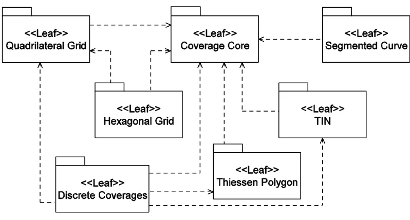
5.2 The coverage schema

(17)

Figure 1 — Packages of the coverage schema

Table 3 — Documentation of coverage geometry packages

Package Clause

Coverage core 5 Discrete coverages 6 Thiessen polygon 7 Quadrilateral grid 8 Hexagonal grid 9

TIN 10

Segmented curve 11

5.3 CV_Coverage

5.3.1 General

The class CV_Coverage (Figure 2) is an instance of the metaclass GF_FeatureType (ISO 19109), which therefore represents a feature type. CV_Coverage shall support three attributes, five operations, and three associations.

5.3.2 domainExtent

The attribute domainExtent[1..*]EX_Extent shall contain the extent of the domain of the coverage. The data type EX_Extent is defined in ISO 19115:2003. Extents may be specified in space, time or space-time.

5.3.3 rangeType

(18)

5.3.4 commonPointRule

The attribute commonPointRule: CV_CommonPointRule shall identify the procedure to be used for evaluating the CV_Coverage at a position that falls either on a boundary between geometric objects or within the boundaries of two or more overlapping geometric objects, where the geometric objects are either CV_DomainObjects or CV_ValueObjects. The data type CV_CommonPointRule is defined in 5.6.

5.3.5 list

The operation list(): Set CV_GeometryValuePair shall return the dictionary of CV_GeometryValuePairs (5.8) that contain the CV_DomainObjects in the domain of the CV_Coverage each paired with its record of feature attribute values. In the case of an analytical coverage, the operation shall return the empty set.

5.3.6 select

The operation select (s: GM_Object, t: TM_Period): Set CV_GeometryValuePair shall accept a GM_Object and a TM_Period as input and return the set of CV_GeometryValuePairs that contain CV_DomainObjects that lie within that GM_Object and TM_Period. If s is null, the operation shall return all CV_GeometryValuePairs that contain CV_DomainObjects within t. If the value of t is null, the operation shall return all CV_GeometryValuePairs that contain CV_DomainObjects within s. In the case of an analytical coverage, the operation shall return the empty set.

5.3.7 find

The operation find (p: DirectPosition, limit: Integer = 1): Sequence CV_GeometryValuePair shall accept a DirectPosition as input and return the sequence of CV_GeometryValuePairs that includes the CV_DomainObjects nearest to the DirectPosition and their distances from the DirectionPosition. The sequence shall be ordered by distance from the DirectPosition, beginning with the Record containing the CV_DomainObject nearest to the DirectPosition. The length of the sequence (the number of CV_GeometryValuePairs returned) shall be no greater than the number specified by the parameter limit. The default shall be to return a single CV_GeometryValuePair. The operation shall return a warning if the last CV_DomainObject in the sequence is at a distance from the DirectPosition equal to the distance of other CV_DomainObjects that are not included in the sequence. In the case of an analytical coverage, the operation shall return the empty set.

NOTE This operation is useful when the domain of a coverage does not exhaustively partition the extent of the coverage. Even in that case, the first element of the sequence returned may be the CV_GeometryValuePair that contains the input DirectPosition.

5.3.8 evaluate

The operation evaluate(p: DirectPosition, list: Sequence CharacterString): Set Record shall accept a DirectPosition as input and return a set of Records of feature attribute values for that direct position. The parameter list is a sequence of feature attribute names each of which identifies a field of the rangeType. If list is null, the operation shall return a value for every field of the rangeType. Otherwise, it shall return a value for each field included in list. The data type DirectPosition is defined in ISO 19107:2003; the data type Record is defined in ISO/TS 19103. If the direct position passed is not in the domain of the coverage, then an error message shall be generated. If the input DirectPosition falls within two or more geometric objects within the domain, the operation shall return records of feature attribute values computed according to the value of the attribute commonPointRule.

(19)

Figure 2 — CV_Coverage

5.3.9 evaluateInverse

The operation evaluateInverse (v: Record): Set CV_DomainObject shall accept a Record of feature attribute values as input and return a set of CV_DomainObjects. Normally, this will be the set of CV_DomainObjects in the Domain that are associated with values equal to those in the input Record. However, the operation may return other CV_DomainObjects derived from those in the domain, as specified by the application schema.

EXAMPLE The evaluateInverse operation could return a set of contours derived from the feature attribute values associated with the CV_GridPoints of a CV_GridCoverage.

5.3.10 Coordinate Reference System

The association Coordinate Reference System shall link the CV_Coverage to the coordinate reference system to which the objects in its domain are referenced. The class SC_CRS is specified in ISO 19111:2003. The multiplicity of the CRS role in the Coordinate Reference System association is one, so a coverage with the same range but with its domain defined in a different coordinate reference system is a different coverage.

5.3.11 Domain

(20)

5.3.12 Range

The association Range shall link the CV_Coverage to the set of CV_AttributeValues in the range. The range of a CV_Coverage shall be a homogeneous collection of records. That is, the range shall have a constant dimension over the entire domain, and each field of the record shall provide a value of the same attribute type over the entire domain.

NOTE This International Standard does not specify how the Domain and Range associations are to be implemented. The relevant data may be generated in real time, it may be held in persistent local storage, or it may be electronically accessible from remote locations.

5.4 CV_DomainObject

5.4.1 General

CV_DomainObject represents an element of the domain of the CV_Coverage. It is an aggregation of objects that may include any combination of GM_Objects (ISO 19107:2003), TM_GeometricPrimitives (ISO 10108), or spatial or temporal objects defined in other standards, such as the CV_GridPoint defined in this International Standard.

5.4.2 SpatialComposition

The association SpatialComposition shall associate a CV_DomainObject to the set of GM_Objects of which it is composed.

5.4.3 TemporalComposition

The association TemporalComposition shall associate a CV_DomainObject to the set of TM_GeometricPrimitives of which it is composed.

5.5 CV_AttributeValues

5.5.1 General

CV_AttributeValues represents an element from the range of the CV_Coverage.

5.5.2 values

The attribute values is a Record containing one value for each attribute, as specified in CV_Coverage.rangeType (5.3.3).

EXAMPLES A coverage with a single (scalar) value (such as elevation). A coverage with a series (array/tensor) of values all defined in the same way (such as brightness values in different parts of the electromagnetic spectrum).

5.5.3 Range

The association Range shall link the set of CV_AttributeValues to the CV_Coverage that has the set as its range (5.3.12).

In the case of a discrete coverage, the multiplicity of CV_Coverage.rangeElement equals that of CV_Coverage.domainElement. In other words, there is one instance of CV_AttributeValues for each instance of CV_DomainObject. Usually, these are stored values that are accessed by the evaluate operation.

(21)

5.6 CV_CommonPointRule

CV_CommonPointRule is a list of codes that identify methods for handling cases where the DirectPosition input to the evaluate operation falls within two or more of the geometric objects. The interpretation of these rules differs between discrete and continuous coverages. In the case of a discrete coverage, each CV_GeometryValuePair provides one value for each attribute. The rule is applied to the set of values associated with the set of CV_GeometryValuePairs that contain the DirectPosition. In the case of a continuous coverage, a value for each attribute shall be interpolated for each CV_ValueObject that contains the DirectPosition. The rule shall then be applied to the set of interpolated values for each attribute. The codes and their meanings are:

a) average – return the mean of the feature attribute values;

b) low – use the least of the feature attribute values;

c) high – use the greatest of the feature attribute values;

d) all – return all the feature attribute values that can be determined for the input DirectPosition;

e) start – use the startValue of the second CV_ValueSegment;

f) end – use the endValue of the first CV_ValueSegment.

NOTE The codes ―start‖ and ―end‖ apply only to segmented curve coverages.

5.7 CV_DiscreteCoverage

5.7.1 General

Figure 3 describes the principal subclasses of CV_Coverage. CV_DiscreteCoverage is the subclass that returns the same record of feature attribute values for any direct position within a single CV_DomainObject in its domain. Subclasses of CV_DiscreteCoverage are described in Clause 6.

5.7.2 locate

The operation locate (p: DirectPosition): Set CV_GeometryValuePair shall accept a DirectPosition as input and return the set of CV_GeometryValuePairs that include CV_DomainObjects containing the DirectPosition. It shall return a null value if the DirectPosition is not on any of the CV_DomainObjects within the domain of the CV_DiscreteCoverage.

5.7.3 evaluate

The operation evaluate (p: DirectPosition, list: Sequence CharacterString): Set Record, which is inherited from CV_Coverage, shall accept a DirectPosition as input, locate the CV_GeometryValuePairs that include the CV_DomainObjects that contain the DirectPosition, and return a set of records of feature attribute values. Normally, the input DirectPosition will fall within only one CV_GeometryValuePair, and the operation will return the record of feature attribute values associated with that CV_GeometryValuePair. If the DirectPosition falls on the boundary between two CV_GeometryPairs, or within two or more overlapping CV_GeometryValuePairs, the operation shall return a record of feature attribute values derived according to the value of the attribute commonPointRule. It shall return a null value if the DirectPosition is not on any of the CV_DomainObjects within the domain of the CV_DiscreteCoverage.

(22)

5.7.5 CoverageFunction

The association CoverageFunction shall link the CV_DiscreteCoverage to the set of CV_GeometryValuePairs included in the coverage.

Figure 3 — CV_Coverage subclasses

5.8 CV_GeometryValuePair

5.8.1 General

The class CV_GeometryValuePair describes an element of a set that defines the relationships of a discrete coverage. Each member of this class consists of two parts: a domain object from the domain of the coverage to which it belongs and a record of feature attribute values from the range of the coverage to which it belongs. CV_GeometryValuePairs may be generated in the execution of an evaluate operation, and need not be persistent. CV_GeometryValuePair is subclassed (Clause 6) to restrict the pairing of a feature attribute value record to a specific subtype of domain object.

5.8.2 geometry

The attribute geometry: CV_DomainObject shall hold the CV_DomainObject that is a member of this CV_GeometryValuePair.

5.8.3 value

(23)

The association CoverageFunction shall link this CV_GeometryValuePair with the CV_DiscreteCoverage of which it is an element.

CV_ContinuousCoverage is the subclass of CV_Coverage that returns a distinct record of feature attribute values for any direct position within its domain.

5.9.2 interpolationType

The attribute interpolationType [0..1]: CV_InterpolationMethod shall be a code that identifies the interpolation method that shall be used to derive a feature attribute value at any direct position within the CV_ValueObject. The attribute is optional – no value is needed for an analytical coverage (one that maps direct position to attribute value by using a mathematical function rather than by interpolation).

5.9.3 interpolationParameterTypes

Although many interpolation methods use only the values in the coverage range as input to the interpolation function, there are some methods that require additional parameters. The optional attribute interpolationParameterTypes specifies the types of parameters that are needed to support the interpolation method identified by interpolationType. The data type RecordType is specified in ISO/TS 19103. It is a dictionary of names and data types.

5.9.4 locate

The operation locate (p: DirectPosition): Set CV_ValueObject shall accept a DirectPosition as input and return the set of CV_ValueObjects that contains this DirectPosition. It shall return a null value if the DirectPosition is not in any of the CV_ValueObjects within the domain of the CV_DiscreteCoverage.

5.9.5 select

The operation select is inherited from CV_Coverage (5.3.6). In the case of CV_ContinuousCoverage, the CV_DomainObjects that shall be returned are those belonging to the CV_GeometryValuePairs associated with the CV_Value Objects of which the CV_ContinuousCoverage is composed.

5.9.6 evaluate

(24)

The operation evaluateInverse (v: record): Set CV_DomainObject, which is inherited from CV_Coverage, shall accept a Record of feature attribute values as input, locate the CV_GeometryValuePairs for which value equals the input record, and return the set of CV_DomainObjects belonging to those CV_GeometryValuePairs. Normally, the CV_DomainObjects that shall be returned are those belonging to the CV_GeometryValuePairs associated with the CV_Value Objects of which the CV_ContinuousCoverage is composed. However, the operation may return other CV_DomainObjects derived from those in the domain, as specified by the application schema. The operation shall return a null value if none of the CV_GeometryValuePairs associated with the CV_DiscreteCoverage has a value equal to the input Record.

EXAMPLE The evaluateInverse operation could return a set of contours derived from the feature attribute values associated with the CV_GridPoints of a CV_GridCoverage.

The association CoverageFunction shall link this CV_ContinuousCoverage to the set of CV_ValueObjects used to evaluate the coverage. This association is optional – an analytical coverage needs no CV_ValueObjects.

5.10 CV_ValueObject

5.10.1 General

CV_ValueObject provides a basis for interpolating feature attribute values within a CV_ContinuousCoverage. CV_ValueObjects may be generated in the execution of an evaluate operation, and need not be persistent.

5.10.2 geometry

The attribute geometry: CV_DomainObject is a CV_DomainObject constructed from the CV_DomainObjects of the CV_GeometryValuePairs that are linked to this CV_ValueObject by the association Control.

5.10.3 interpolationParameters

The optional attribute interpolationParameters: Record shall hold the values of the parameters required to execute the interpolate operation, as specified by the interpolationParameterTypes attribute of CV_ContinuousCoverage.

5.10.4 interpolate

The operation interpolate (p: DirectPosition): Record shall accept a DirectPosition as input and return the record of feature attribute values computed for that DirectPosition.

5.10.5 Control

The association Control shall link this CV_ValueObject to the set of CV_GeometryValuePairs that provide the basis for constructing the CV_ValueObject and for evaluating the CV_ContinuousCoverage at DirectPositions within this CV_ValueObject.

(25)

5.11 CV_InterpolationMethod

CV_InterpolationMethod is a list of codes that identify interpolation methods that may be used for evaluating continuous coverages. See Annex C for descriptions of specific interpolation methods.

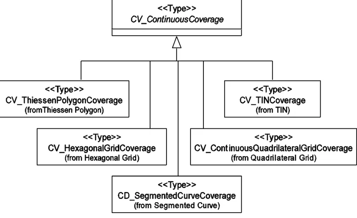
5.12 Subclasses of CV_ContinuousCoverage

This International Standard specifies schemas for five subclasses of CV_ContinuousCoverage (Figure 4). CV_ThiessenPolygonCoverage is specified in Clause 7, CV_ContinuousQuadrilateralGridCoverage is specified in Clause 8, CV_HexagonalGridCoverage is specified in Clause 9, CV_TINCoverage is specified in Clause 10, and CV_SegmentedCurveCoverage is specified in Clause 11.

Figure 4 — Continuous coverages

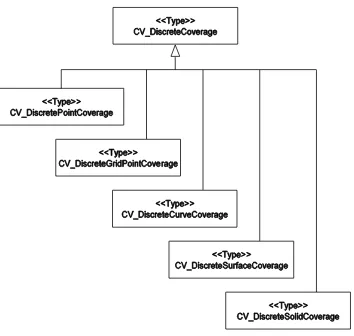
6 Discrete coverages

6.1 Discrete coverage types

(26)

Figure 5 — Discrete coverage types

Because the superclass is not abstract, an instance of the superclass may consist of mixed types of CV_GeometryValuePair.

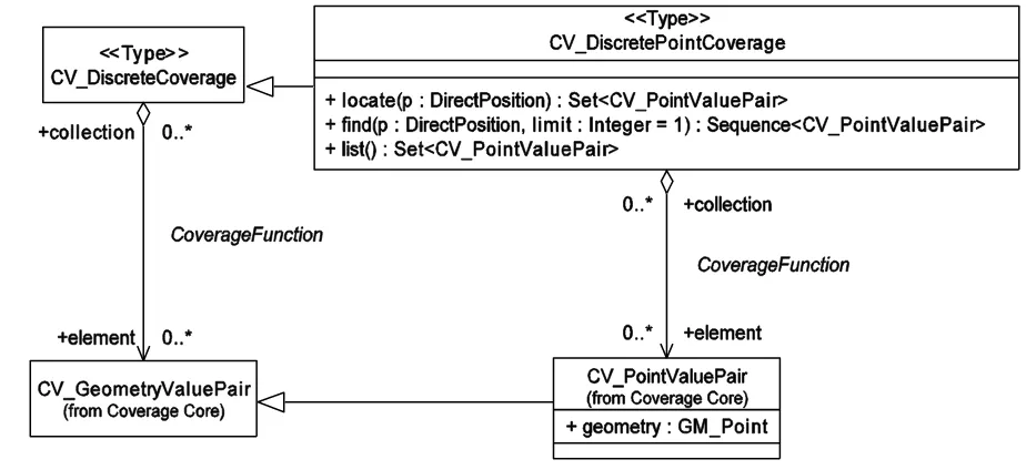
6.2 CV_DiscretePointCoverage

6.2.1 General

A discrete point coverage is characterized by a finite domain consisting of points. Generally, the domain is a set of irregularly distributed points. However, the principal use of discrete point coverages is to provide a basis for continuous coverage functions, where the evaluation of the continuous coverage function is accomplished by interpolation between the points of the discrete point coverage. Most interpolation algorithms depend upon a structured pattern of spatial relationships between the points. This requires either that the points in the spatial domain of the discrete point coverage be arranged in a regular way, or that the spatial domain of the continuous coverage be partitioned in a regular way in relation to the points of the discrete point coverage. Grid coverages (Clauses 8 and 9) employ the first method; Thiessen polygon (Clause 7) and TIN (Clause 10) coverages employ the second.

(27)

Figure 6 — CV_DiscretePointCoverage

6.2.2 Inherited associations and operations

CV_DiscretePointCoverage (Figure 6) inherits the association CoverageFunction and the operations locate, find, and list from CV_DiscreteCoverage (5.7), with the restriction that the associated CV_GeometryValuePairs and those returned by the operations shall be limited to CV_PointValuePairs.

6.3 CV_PointValuePair

CV_PointValuePair is the subtype of CV_GeometryValuePair that has a GM_Point as the value of its geometry attribute.

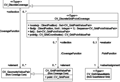
6.4 CV_DiscreteGridPointCoverage

6.4.1 General

The domain of a CV_DiscreteGridPointCoverage (Figure 7) is a set of CV_GridPoints (8.5) that are associated with records of feature attribute values through a CV_GridValuesMatrix (8.14).

6.4.2 Inherited associations and operations

(28)

Figure 7 — CV_DiscreteGridPointCoverage

6.4.3 point

The operation point (g: CV_GridCoordinates): CV_GridPointValuePair shall accept a grid coordinate as input and use data from the associated CV_GridValuesMatrix to construct and return the CV_GridPointValuePair associated with that grid position.

6.4.4 PointFunction

The association PointFunction shall link the CV_DiscreteGridPointCoverage to the CV_GridValuesMatrix for which it is an evaluator.

6.5 CV_GridPointValuePair

CV_GridPointValuePair is the subtype of CV_GeometryValuePair that has a GM_GridPoint as the value of its geometry attribute.

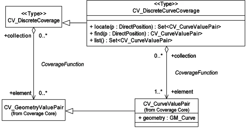
6.6 CV_DiscreteCurveCoverage

6.6.1 General

A discrete curve coverage is characterized by a finite spatial domain consisting of curves. Often the curves represent features such as roads, railroads or streams. They may be elements of a network.

(29)

6.6.2 Inherited operations and associations

CV_DiscreteCurveCoverage (Figure 8) inherits the association CoverageFunction and the operations locate, find, list, evaluate and evaluateInverse from CV_DiscreteCoverage, with the restriction that the associated CV_GeometryValuePairs and those returned by the operations shall be limited to CV_CurveValuePairs.

Figure 8 — CV_DiscreteCurveCoverage

6.7 CV_CurveValuePair

CV_CurveValuePair is the subtype of CV_GeometryValuePair that has a GM_Curve as the value of its geometry attribute.

6.8 CV_DiscreteSurfaceCoverage

6.8.1 General

A discrete surface coverage is a coverage whose domain consists of a collection of surfaces. In most cases, the surfaces that constitute the domain of a coverage are mutually exclusive and exhaustively partition the extent of the coverage. Surfaces or their boundaries may be of any shape. The boundaries of component surfaces often correspond to natural phenomena and are highly irregular.

EXAMPLE A coverage that represents soil types typically has a spatial domain composed of surfaces with irregular boundaries.

(30)

Figure 9 — CV_DiscreteSurfaceCoverage

CV_DiscreteSurfaceCoverage (Figure 9) inherits the association CoverageFunction and the operations locate, find, list, evaluate, and evaluateInverse from CV_DiscreteCoverage, with the restriction that the associated CV_GeometryValuePairs and those returned by the operations shall be limited to CV_SurfaceValuePairs.

6.8.3 TINBase

The association TINBase may be used to link a CV_DiscreteSurfaceCoverage to a CV_TINCoverage (10.2). The constraint

discreteTIN.element.geometry = triangleSource.controlValue.geometry

requires that the spatial domain of the CV_DiscreteSurfaceCoverage be composed of the triangles belonging to the CV_TINCoverage.

6.8.4 ThiessenBase

The association ThiessenBase may be used to link a CV_DiscreteSurfaceCoverage to a CV_ThiessenPolygonCoverage (7.2). The constraint

discreteThiessen.element.geometry = polygonSource.controlValue.geometry

(31)

6.9 CV_SurfaceValuePair

CV_SurfaceValuePair is the subtype of CV_GeometryValuePair that has a GM_Surface as the value of its geometry attribute.

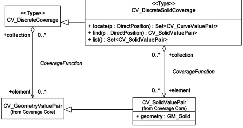
6.10 CV_DiscreteSolidCoverage

6.10.1 General

A discrete solid coverage is a coverage whose domain consists of a collection of solids. Solids or their boundaries may be of any shape. Generally, the solids that constitute the domain of a coverage are mutually exclusive and exhaustively partition the extent of the coverage, but this is not required.

EXAMPLE Buildings in an urban area could be represented as a set of unconnected GM_Solids each with attributes such as building name, address, floor space and number of occupants.

As in the case of surfaces (5.8), the spatial domain of a discrete solid coverage may be a regular or semiregular tessellation of the extent of the coverage. The tessellation can be defined in terms of a three-dimensional grid, where the set of grid cells is the spatial domain of the coverage.

Figure 10 — CV_DiscreteSolidCoverage

CV_DiscreteSolidCoverage (Figure 10) inherits the association CoverageFunction and the operations locate, find, list, evaluate and evaluateInverse from CV_DiscreteCoverage, with the restriction that the associated CV_GeometryValuePairs and those returned by the operations shall be limited to CV_SolidValuePairs.

6.11 CV_SolidValuePair

(32)

7 Thiessen polygon coverage

7.1 Thiessen polygon networks

A finite collection of points on a plane determines a partition of the plane into a collection of polygons equal in number to the collection of points. A Thiessen polygon is generated from one of a defining set of points by forming the set of direct positions that are closer to that point than to any other point in the defining set. The specific point is called the centre of the resulting polygon. The boundaries between neighbouring polygons are the perpendicular bisectors of the lines between their respective centres. Each polygon shares each of its edges with exactly one other polygon. Each polygon contains exactly one point from the defining set. Thiessen polygons are also known as Voronoi Diagrams or Proximal Sets.

Figure 11 — An example of a Thiessen polygon network with (x,y) coordinates

A Thiessen polygon network (Figure 11) is a tessellation of a two-dimensional space using Thiessen Polygons. A Thiessen polygon network provides a structure that supports interpolation of feature attribute values from the polygon centres to direct positions within the polygons.

EXAMPLE Figure 11 shows a collection of points with their (x,y) coordinates, the perpendicular bisectors of the lines that would be drawn between them, and the resultant polygons.

7.2 CV_ThiessenPolygonCoverage

7.2.1 General

A CV_ThiessenPolygonCoverage (Figure 12) evaluates a coverage at direct positions within a Thiessen polygon network constructed from a set of discrete point value pairs. Evaluation is based on interpolation between the centres of the CV_ThiessenValuePolygons surrounding the input position.

7.2.2 clipArea

(33)

7.2.3 interpolationType

The inherited attribute interpolationType: CV_InterpolationMethod = “lost area” shall identify the interpolation method to be used in evaluating the coverage. The most common interpolation methods are ―lost area‖ (C.9) and ―nearest neighbour‖ (C.2). Lost area interpolation can return a different Record of feature attribute values for each direct position within a CV_ThiessenValuePolygon. On the other hand, nearest neighbour interpolation will return for any direct position within a CV_ThiessenValuePolygon the Record associated with the CV_PointValuePair at the centre of the CV_ThiessenPolygon. In other words, a CV_ThiessenPolygonCoverage that uses nearest neighbour interpolation acts like a discrete surface coverage.

7.2.4 locate

The operation locate (p: DirectPosition): CV_ThiessenValuePolygon is inherited from CV_ContinuousCoverage with the restriction that it shall return a CV_ThiesenValuePolygon. It shall accept a DirectPosition as input and return the CV_ThiessenValuePolygon that contains that DirectPosition.

Figure 12 — CV_ThiessenPolygonCoverage

7.2.5 evaluate

(34)

The association CoverageFunction shall link this CV_ThiessenPolygonCoverage to the CV_ThiessenValuePolygons of which it is composed.

7.3 CV_ThiessenValuePolygon

7.3.1 General

CV_ThiessenValuePolygon is a subclass of CV_ValueObject. Individual CV_ThiessenValuePolygons may be generated during the evaluation of a CV_ThiessenPolygonCoverage, and need not be persistent.

7.3.2 geometry

The attribute geometry:GM_Polygon shall hold the geometry of the Thiessen polygon centred on the CV_PointValuePair identified by the association Control.

7.3.3 Control

The association Control shall link this CV_ThiessenValuePolygon to the CV_PointValuePair at its centre.

8 Quadrilateral grid coverages

8.1 General

Grid coverages employ a systematic tessellation of the domain. The principal advantage of such tessellations is that they support a sequential enumeration of the elements of the domain, which makes data storage and access more efficient. The tessellation may represent how the data were acquired or how they were computed in a model. The domain of a grid coverage is a set of grid points, including their convex hull in the case of a continuous grid coverage.

8.2 Quadrilateral grid geometry

8.2.1 General

A grid is a network composed of two or more sets of curves in which the members of each set intersect the members of the other sets in a systematic way. The curves are called grid lines; the points at which they intersect are grid points, and the interstices between the grid lines are grid cells.

(35)

Figure 13 — Example — A 7  7 two-dimensional orthogonal grid

NOTE The dimensions (axes) of a 2-dimensional grid are often called row and column.

A grid may be defined in terms of an external coordinate reference system. This requires additional information about the location of the grid’s origin within the external coordinate reference system, the orientation of the grid axes, and a measure of the spacing between the grid lines. If the spacing is uniform, then there is an affine relationship between the grid and external coordinate system, and the grid (Figure 14) is called a rectified grid. If, in addition, the external coordinate reference system is related to the earth by a datum, the grid is a georectified grid. The grid lines of a rectified grid need not meet at right angles; the spacing between the grid lines is constant along each axis, but need not be the same on every axis. The essential point is that the transformation of grid coordinates to coordinates of the external coordinate reference system is an affine transformation.

NOTE 1 The word rectified implies a transformation from an image space to another coordinate reference system. However, grids of this form are often defined initially in an earth-based coordinate system and used as a basis for collecting data from sources other than imagery.

NOTE 2 The internal grid coordinate system is an instance of an engineering coordinate reference system as specified by ISO 19111:2003. Its datum is a set of one or more ground control points.

Key

X, Y, Z axes to determine 3-space V₁, V₂ offset vectors

0 grid origin

(36)

EXAMPLE Figure 14 shows a two-dimensional grid in the 3-space determined by the axes X, Y, and Z. The grid origin is at O. There are two offset vectors labelled V₁ and V₂ which specifythe orientation of the grid axes and the spacing between the grid lines. The coordinates of the grid points are of the form: O + aV₁ + bV₂.

When the relationship between a grid and an external coordinate reference system is not adequate to specify it in terms of an origin, an orientation and spacing in that coordinate reference system, it may still be possible to transform the grid coordinates into coordinates in the coordinate reference system. This transformation need not be in analytic form; it may be a table, relating the grid points to coordinates in the external coordinate reference system. Such a grid is classified as a referenceable grid. If the external coordinate reference system is related to the earth by a datum, the grid is a georeferenceable grid. A referenceable grid is associated with information that allows the location of all points in the grid to be determined in the coordinate reference system, but the location of the points is not directly available from the grid coordinates, as opposed to a rectified grid where the location of the points in the coordinate reference system is derivable from the properties of the grid itself. The transformation produced by the information associated with a referenceable grid will produce a grid as seen in the coordinate reference system, but the grid lines of that grid need not be straight or orthogonal, and the grid cells may be of different shapes and sizes.

8.2.2 Cell structures

The term ―grid cell‖ refers to two concepts: one important from the perspective of data collection and portrayal, the other important from the perspective of grid coverage evaluation. The ambiguity of this term is a common cause of positioning error in evaluating or portraying grid coverages.

The feature attribute values associated with a grid point represent characteristics of the real world measured or observed within a small space surrounding a sample point represented by the grid point. The grid lines connecting these points form a set of grid cells. A common simplifying assumption is that the sample space is equally divided among the sample points, so that the sample spaces are represented by a second set of cells congruent to the first, but offset so that each has a grid point at its centre. Evaluation of a grid coverage is based on interpolation between grid points, i.e. within a grid cell bounded by the grid lines that connect the grid points that represent the sample points.

Key

a, b, c, d grid points

A, B, C, D cells (bounded by dotted lines) U grid cell (bounded by solid lines) X direct position within the grid cell

Figure 15 — Grid cell structures

(37)

direct position X within the grid cell U (bounded by the solid lines) will be based on interpolation from a, b, c and d (and possibly involve additional grid points outside the cell).

In this International Standard, the term grid cell refers to the cell bounded by the grid lines that connect the grid points. The term sample space refers to the observed or measured space surrounding a sample point. The term footprint refers to a representation of a sample space in the context of some coordinate reference system.

In dealing with gridded data, e.g. for processing or portrayal, it is often assumed that the size and shape of the sample spaces are a simple function of the spatial distribution of the sample points, and that the grid cells and the sample cells are congruent.

In fact, the size and shape of the sample space are determined by the method used to measure or calculate the attribute value. In the simplest case, the sample space is the sample point. It is often a disc, a sphere, or a hypersphere surrounding the sample point. In the case of sensed data, the size and shape of the sample space is also a function of the sensor model and its position relative to the sample point, and may be quite complex. Adjacent sample spaces may be coterminous or they may overlap or underlap.

In addition to affecting the size and shape of the sample space, the measurement technique affects the applicability of the observed or measured value to the sample space. It is often assumed that the recorded value represents the mean value for the sample space. In fact, elements of the sample space may not contribute uniformly to the result, so that it is better conceived as a weighted average where the weighting is a function of position within the sample space. Interpolation methods may be designed specifically to deal with characteristics of the sample space.

Transformation (e.g. rectification) between grid coordinates and an external coordinate reference system may distort the representation of the sample space in a way that causes interpolation errors.

8.3 CV_Grid

8.3.1 General

(38)

Figure 16 — CV_Grid 8.3.2 dimension

The attribute dimension: Integer shall identify the dimensionality of the grid.

8.3.3 axisNames

The attribute axisNames: Sequence CharacterString shall list the names of the grid axes.

8.3.4 extent

The optional attribute extent: CV_GridEnvelope shall specify the limits of a section of the grid.

8.3.5 Organization

The association Organization shall link the CV_Grid to the set of CV_GridPoints that are located at the intersections of the grid lines.

8.3.6 EvaluationStructure

The association EvaluationStructure shall link the CV_Grid to the set of CV_GridCells delineated by the grid lines.

8.3.7 Subclasses

(39)

CV_GridValuesMatrix (8.14), which contains information for assigning values from the range to each of the grid points.

CV_Grid is not an abstract class: an instance of CV_Grid need not be an instance of any of its subclasses. The partitions indicate that an instance of the subclass CV_GridValuesMatrix may be, at the same time, an instance of either the subclass CV_RectifiedGrid or of the subclass CV_ReferenceableGrid.

8.4 CV_GridEnvelope

8.4.1 General

CV_GridEnvelope (Figure 16) is a data type that provides the grid coordinate values for the diametrically opposed corners of the CV_Grid. It has two attributes, low and high.

8.4.1.1 low

CV_GridPoint is the class that represents the intersections of the grid lines.

8.5.2 gridCoord

The attribute gridCoord: CV_GridCoordinate holds the set of grid coordinates that specifies the location of the CV_GridPoint within the CV_Grid.

8.5.3 Organization

The association Organization shall link the CV_GridPoint to the CV_Grid of which it is an element.

8.5.4 Location

The association Location shall link the CV_GridPoint to the set of CV_GridCells for which it is a corner. The multiplicity at the CV_GridPoint end of the association has no upper bound, to allow for grids of any dimension. In a quadrilateral grid, the multiplicity of corner equals 2d_{, where}d_{is the value of CV_Grid.dimension.}

8.5.5 Reference

The association Reference may link the CV_GridPoint to the GM_Point that is its representation in an external coordinate reference system.

8.5.6 SampleSpace

(40)

8.6 CV_GridCoordinate

8.6.1 General

CV_GridCoordinate is a data type for holding the grid coordinates of a CV_GridPoint.

8.6.2 coordValues

The attribute coordValues: Sequence Integer shall hold one integer value for each dimension of the grid. The ordering of these coordinate values shall be the same as that of the elements of CV_Grid.axisNames. The value of a single coordinate shall be the number of offsets from the origin of the grid in the direction of a specific axis.

8.7 CV_GridCell

8.7.1 General

A CV_GridCell is delineated by the grid lines of CV_Grid. Its corners are associated with the CV_GridPoints at the intersections of the grid lines that bound it.

8.7.2 Location

The association Location shall link the CV_GridCell to the set of CV_GridPoints at its corners.

8.7.3 EvaluationStructure

The association EvaluationStructure shall link the CV_GridCell to the CV_Grid of which it is a component.

8.8 CV_Footprint

8.8.1 General

A CV_Footprint is the sample space of a grid in an external coordinate reference system.

8.8.2 geometry

The attribute geometry: GM_Object shall describe the geometry of the CV_Footprint within the coordinate reference system identified by GM_Object.CRS (ISO 19107:2003).

8.8.3 SampleSpace

(41)

Figure 17 — CV_Grid subclasses

8.9 CV_RectifiedGrid

8.9.1 General

A rectified grid shall be defined by an origin in an external coordinate reference system, and a set of offset vectors that specify the direction and distance between the grid lines within that external coordinate reference system (Figure 14).

The class CV_RectifiedGrid (Figure 17) contains the additional geometric characteristics of a rectified grid.

8.9.2 origin

The attribute origin: DirectPosition is a direct position that shall locate the origin of the rectified grid in an external coordinate reference system. That coordinate reference system is identified through the association Coordinate Reference System (specified in ISO 19107:2003) between DirectPosition and the class SC_CRS specified in ISO 19111:2003.

8.9.3 offsetVectors

(42)

8.9.4 coordConv

The operation coordConv (g: CV_GridCoordinate): DirectPosition shall accept a CV_GridCoordinate as input and return a DirectPosition. The operation uses the values of the attributes origin and offsetVectors in an affine transformation. It is a coordinate conversion operation as defined by ISO 19111:2003.

8.9.5 invCoordConv

The operation invCoordConv (p: DirectPosition): CV_GridCoordinate shall accept a DirectPosition as input and return the CV_GridCoordinate of the nearest CV_GridPoint. The operation uses the values of the attributes origin and offsetVectors in an affine transformation. It is a coordinate conversion operation as defined by ISO 19111:2003.

8.9.6 Constraints

a) dimension = origin.CRS.theSC_CoordinateSystem.dimension The dimension of the grid shall be less than or equal to the dimension of the coordinate reference system identified through the Coordinate Reference System association of the GM_Point that is the origin.

b) offsetVectors  size = dimension The number of offset vectors shall equal the dimension of the grid.

c) offsetVectors-forAll(dimension = self.origin.CRS.theSC_CoordinateSystem.dimension) The dimension of the offset vectors shall equal the dimension of the coordinate reference system, even if an offset vector is aligned with an axis of the external coordinate system.

8.10 CV_ReferenceableGrid

8.10.1 General

CV_ReferenceableGrid shall support two operations, coordTransform and invCoordTransform.

8.10.1.1 coordTransform

The operation coordTransform (g: CV_GridCoordinate): DirectPosition shall accept a CV_GridCoordinate as input and return a DirectPosition in the coordinate reference system identified through the association Coordinate Reference System (8.10.2). This is a coordinate transformation operation as defined by ISO 19111:2003.

8.10.1.2 invCoordTransform

The operation invCoordConv (p: DirectPosition): CV_GridCoordinate shall accept a DirectPosition in the coordinate reference system identified through the association Coordinate Reference System (8.10.2) as input and return the CV_GridCoordinate of the nearest CV_GridPoint. This is a coordinate transformation operation as defined by ISO 19111:2003.

8.10.2 Coordinate Reference System