INTEGRATED PROCESSING OF HIGH RESOLUTION TOPOGRAPHIC DATA FOR
SOIL EROSION ASSESSMENT CONSIDERING DATA ACQUISITION SCHEMES AND
SURFACE PROPERTIES
A. Eltner a*, D. Schneider a, H.-G. Maas a
a Technische Universität Dresden, Institute of Photogrammetry and Remote Sensing, 01016 Dresden, Germany - (Anette.Eltner, Danilo.Schneider, Hans-Gerd.Maas)@tu-dresden.de
Commission V, WG V/5
KEY WORDS: UAV photogrammetry, TLS, data fusion, scan geometry, surface roughness, soil erosion
ABSTRACT:
Soil erosion is a decisive earth surface process strongly influencing the fertility of arable land. Several options exist to detect soil erosion at the scale of large field plots (here 600 m²), which comprise different advantages and disadvantages depending on the applied method. In this study, the benefits of unmanned aerial vehicle (UAV) photogrammetry and terrestrial laser scanning (TLS) are exploited to quantify soil surface changes. Beforehand data combination, TLS data is co-registered to the DEMs generated with UAV photogrammetry. TLS data is used to detect global as well as local errors in the DEMs calculated from UAV images. Additionally, TLS data is considered for vegetation filtering. Complimentary, DEMs from UAV photogrammetry are utilised to detect systematic TLS errors and to further filter TLS point clouds in regard to unfavourable scan geometry (i.e. incidence angle and footprint) on gentle hillslopes. In addition, surface roughness is integrated as an important parameter to evaluate TLS point reliability because of the increasing footprints and thus area of signal reflection with increasing distance to the scanning device. The developed fusion tool allows for the estimation of reliable data points from each data source, considering the data acquisition geometry and surface properties, to finally merge both data sets into a single soil surface model. Data fusion is performed for three different field campaigns at a Mediterranean field plot. Successive DEM evaluation reveals continuous decrease of soil surface roughness, reappearance of former wheel tracks and local soil particle relocation patterns.
1. INTRODUCTION
Soil erosion is an important process influencing the fertility of the earth surface, which is significant regarding its agricultural exploitation. To support the understanding of the process of soil particle relocation, soil surface changes determined with multi-temporal digital elevation models (DEMs) of high spatial resolution and accuracy can be analysed. Thereby, the surface has to remain undisturbed to capture alterations. Furthermore, the investigated plot needs to exceed a minimum size in regard to assess sediment connectivity resulting in possible varying erosion rates (e.g. Bracken et al., 2015). This is especially relevant for soil erosion studies in the Mediterranean, e.g. the fragile marl landscape of Andalusia (Spain) as in this study, where high erosion rates with unique sediment connectivity characteristics are common because of soil properties and climatic conditions (e.g. Cammeraat, 2004, García-Ruiz et al., 2013).
Different high resolution topography measurement methods with varying advantages and disadvantages exist (Passalacqua et al., 2015) to estimate soil erosion at large field plots. More specific, terrestrial laser scanning (TLS) and unmanned aerial vehicle (UAV) photogrammetry as the combination of UAV images with structure from motion (SfM) and multi-view stereo (MVS) dense matching processing can be used. Image based surface reconstruction receives an increasing interest in earth surface studies in recent years (e.g. Eltner et al., 2015a). 1 Point clouds from TLS are reliable in regard to their geometric error behaviour (e.g. Vosselman & Maas, 2010) and may thus be assumed to be useful for the evaluation of DEMs obtained from UAV photogrammetry (UAV DEM). Furthermore, TLS
* Corresponding author
data is considered to more reliably filter vegetation spots (Brodu & Lague, 2012), which may be problematic in UAV data due to difficulties encountered from image matching over plant cover (e.g. Eltner et al., 2015b). However, unfavourable scan geometry due to low viewing angles on the soil surface of gently rolling hills prone to erosion results in fast increasing incidence angles and increasing footprints with increasing distance to the TLS device, leading to increased error probability (e.g. Soudarissanane et al., 2011).
Regarding the performance of TLS, surface roughness (or complexity) is a further factor influencing the accuracy of the point cloud, which is in particular relevant for agriculturally utilised soil surfaces (Barneveld et al., 2013).
Regarding data combination, UAV data inherits limitations, as well. The complex error behaviour during the 3D reconstruction from overlapping images can result in global inaccuracies such as the dome error (e.g. James & Robson, 2014, Eltner & Schneider, 2015) due to error propagation in the image block governed by ground control point (GCP) distribution (Kraus, 2007). In addition, local blunders are possible e.g. due to matching issues over low textured areas. Nevertheless, DEMs reconstructed from overlapping UAV images can be used as independent method to detect and correct for certain systematic TLS errors (as revealed with a total station reference in Eltner & Baumgart, 2015). Furthermore, the UAV DEMs are suitable to evaluate the TLS point quality in regard to the scan geometry allowing for TLS point cloud filtering considering the parameters incidence angle, footprint size and surface roughness, which can be calculated utilising the UAV DEMs and scan positions (SP) of the TLS device.
In this study, a tool is developed for synergetic data fusion
accounting for the advantages and disadvantages of both high resolution topography measurement methods. More specifically, the introduced approach automatically incorporates information about the data acquisition configurations as well as surface properties to utilise the potential of TLS and UAV data, respectively. Subsequently, both high resolution topographic datasets are merged to estimate a precise digital soil surface model.
Concluding, multi-temporal assessment of the processed data is performed for three field campaigns from September 2013 to February 2014 capturing single precipitation events revealing steady soil roughness decrease and locally varying height changes.
2. DATA AQUCISITION AND PROCESSING
2.1 Study area
Selective combination of highly resolved topographic data from different sources is evaluated for an investigation plot in the fragile marl landscape of Andalusia (Spain, Fig. 1a). The region is characterised by high erosion rates due to physical and geochemical soil properties and due to climatic conditions, i.e. torrential precipitation events after dry summers (Poesen & Hooke, 1997, Faust & Schmid, 2009). Thus, detectable soil surface changes are expected during a study period of 5 months. Three field campaigns are conducted during the autumn and rainy winter season (17.09.2013, 01.11.2013, 14.02.2014).
Figure 1. Description of the study site. a) Location of the field plot and setup of multi-temporal reference points (map from IGN Spain, http://www2.ign.es/iberpix/visoriberpix/visorign.html), b) Positions of scanning device during each field campaign and setup of further field proximal reference points.
The area of interest depicts a size of about 20 x 30 m and is located at the upper position of a hillslope within an actively agriculturally utilised field. The plot extent is chosen to capture changes ranging from the micro-plot scale to the field plot scale, which is especially important in this landscape because of a erosion pattern revealing a complex sediment (dis-)connectivity (Faust & Schmid, 2009).
2.2 Methods of high resolution topography
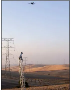
To acquire topographic data with high resolution for precise soil surface change detection, the methodological approaches of TLS and UAV photogrammetry (Fig. 2) were chosen due to their flexible implementation and because they are non-contact methods, especially relevant for area-based, multi-temporal observations.
2.2.1 UAV data: The aerial images were collected with the
UAV “Asctec Falcon 8”, which is an octo-copter micro-drone.
The platform features an active stabilising camera mount
guaranteeing constant viewing directions and compensation of UAV movements due to wind and system-intern vibrations. Images were captured with a compact system camera (Sony NEX-5N) equipped with a fixed focal length (16 mm). The sensor size is 23.5 x 15.6 mm with 4.8 µm pixel size. The UAV acquired the data at flying heights between 8 and 12 m and hence resulting in maximal ground sampling distances of 2.5 mm. In total, about 160 images were taken during each field campaign with an along- and cross-flight strip image overlap of 85 and 75%, respectively.
To retrieve the DEMs from the UAV images, Pix4D was chosen for data processing. This software solution is especially designed for UAV photogrammetry, combining photo-grammetry and computer vision approaches for aerial triangulation and using MVS methods for dense-matching (Küng et al., 2012). In this study, the final DEMs are slightly noise filtered raster with a resolution of 1 cm.
To retrieve the DEMs from the UAV images Pix4D was chosen for data processing. This software solution is especially designed for UAV photogrammetry, combining photo-grammetry and computer vision approaches for aerial triangulation and using MVS methods for dense-matching (Küng et al., 2012). In this study, the final DEMs are slightly noise filtered rasters with a resolution of 1 cm.
2.2.2 TLS data: TLS was conducted with a Riegl LMS-Z420i (installed at a 4 m high tripod), which uses the time-of-flight principle for distance calculation. The scanning device was installed at different positions surrounding the area of interest to compensate for occlusion effects at a rough soil surface (Fig. 1b) – 8 SPs during the first two field campaigns and 6 SPs during the last campaign. The angular resolution was set to an angle that resulted in 4 mm point distance at a scanner-to-object distance of 10 m causing high information redundancy, which is utilised to smooth random errors (e.g. Abellán et al., 2009) in following processing stages. The measurement of soil erosion on gently rolling hillslopes is especially challenging due to low viewing angles at the surface inducing high incidence angles and large footprints, e.g. >60° and >2.5 cm, respectively, at distances >8 m; even though a high tripod has been used to enhance the scan geometry (more detail in Eltner & Baumgart, 2015).
Figure 2. Photo of the applied TLS device and UAV.
2.2.3 Data registration: A stable reference system is a prerequisite for multi-temporal change detection. Therefore, several registration targets (retro-reflective cylinders with white circled markers on top and regular GCPs), which were
especially designed for the data acquisition schemes in this study (Eltner et al., 2013), are measured with a total station (Fig. 1). In total, 5 marking pipes are installed around the field plot until a depth of about 60 cm, at which the registration targets are put during each field campaign. Furthermore, three additional reference points are established at utility poles nearby to backup the targets at the marking pipes because their stability is difficult to assure at an agriculturally worked field with heavy machines passing close by the investigation plot. However, evaluation of the reference consistency by a 3D similarity transformation between the measured marking pipe positions of subsequent field campaigns reveals reliable target stability indicated by movements less than 2.5 mm (Tbl. 1). The reference points at the utility poles are used together with the targets at the marking pipes to adjust the location of temporary points (at least 12 targets), which were laid out around the plot additionally to the 5 installed registration targets for GCP redundancy. Thus, transferring of the temporary points into the local reference system during each field campaign resulted in a maximum error of 2.7 mm (Tbl. 1).
target stability target accuracy in the local reference system lateral vertical lateral vertical
17.09.2013 - - 2.7 mm 0.7 mm
01.11.2013 1.6 mm 1.0 mm 1.0 mm 0.2 mm
14.02.2014 2.4 mm 2.5 mm 1.0 mm 0.6 mm
Table 1. Referencing performance: Target stability as residuals of transformation of measured targets of subsequent campaigns and target accuracy as residuals of transformation into local reference system.
Besides the targets used for multi-temporal assessment, further retro-reflective cylinders were installed behind the SPs. These additional cylinders were not measured by total station and were solely used to enhance the transformation of the point clouds of the single SPs into a project system for each field campaign. They are supposed to increase the performance of a generally weak referencing geometry of the TLS data due to measured target distribution only in-front of the scanning device because GCPs were not possible in larger distances from the plot due to active land cultivation (Eltner & Baumgart, 2015). The transformation into the project system and subsequently into the local system resulted in registration errors of about 5 mm and 6 mm, respectively, whereas registration accuracy of the DEMs from UAV photogrammetry amounts about 4 mm (Tbl. 2).
TLS UAV
project system local system local system
17.09.2013 5.5 mm 5.5 mm 3 mm
01.11.2013 4.9 mm 6.3 mm 4 mm
14.02.2014 5.4 mm 6.1 mm 4 mm
Table 2. Accuracy of data registration of both high resolution topography datasets into corresponding reference systems (TLS data to project system is the average error of all SPs).
2.3 Synergetic data fusion
Point clouds evolving from UAV photogrammetry as well as TLS are combined to a single point cloud in a rule-based approach considering the benefits of each method (Fig. 3). In a preliminary evaluation of the UAV data quality, the TLS data is utilised to detect a potential DEM dome due to parallel-axes UAV image configuration (Eltner & Schneider, 2015) and local DEM blunders due to matching errors, e.g. over surfaces with low texture, which occur frequently after precipitation events that cause sheet erosion and thus homogenisation of soil material. Thereby, corrected, vegetation-filtered, noise-smoothened, and down-sampled TLS data, according to Eltner
& Baumgart (2015), is utilised. Data gaps due to unsuccessful image matching are padded by the TLS data.
Vice versa, UAV DEMs are considered to detect systematic errors in the TLS data calculating the TLS point to UAV mesh distance in CloudCompare (Girardeau-Montaut, 2016). If an error is obvious, the TLS data is corrected via a lookup table (more detail in Eltner & Baumgart, 2015). However, beforehand systematic error retrieval, both high resolution topographic datasets are co-registered with an iterative closest point (ICP; Besl & McKay, 1992) algorithm. Thereby, TLS point clouds of each SP are registered to the corresponding UAV data. The DEMs from UAV photogrammetry are considered more reliable in regard of referencing because sub-pixel measurements of GCPs are realisable and registration targets are well distributed around the area of interest. Whereas, TLS data comprises unfavourable registration geometry and accuracy of registration target measurement is difficult to estimate due to automatic fitting with retro-reflective cylinders (e.g. Pesci & Teza, 2008).
Figure 3. Conceptual workflow for synergetic fusion of data acquired from TLS and UAV photogrammetry (after Eltner, 2016).
UAV DEMs are further exploited to filter the TLS data in regard of scan geometry. Thus, the UAV DEMs are the references to calculate incidence angle (eq. 1, Soudarissanane et al., 2011) and footprint size (eq. 2, e.g. Schürch et al., 2011) considering each SP and the topography, which is smoothed with a moving median filter to eliminate outliers and a moving Gaussian filter to generally reduce data noise.
(1)
where α= incidence angle D = object to scanner vector N = surface normal
(2)
where Flax= footprint size of the long axis d = object to scanner distance
= laser beam divergence b = laser emergence size
Calculated incidence angle and footprint values are assigned to the TLS data using kd-trees and nearest neighbour assignments realised with the point cloud library (PCL; Rusu & Cousins, 2011). Thresholds are defined for a maximum tolerable distance between the topographic reference (UAV DEM) and TLS point, a maximum incidence angle and a maximum footprint.
Furthermore, TLS data is used for vegetation filtering due to the characteristic appearance of vegetation in point clouds acquired from terrestrial perspective, which can be exploited by point based classification approaches, such as CANUPO (Brodu & Lague, 2012). Points in the UAV data, which are below a
defined distance threshold to points that have been identified as vegetation in the TLS point cloud, are filtered. Thus, plant covered spots at the field plot are excluded to avoid erroneous multi-temporal calculations, however, increasing the risk of underestimation of actual surface changes.
Besides the consideration of data acquisition schemes, surface properties, i.e. soil surface roughness, are incorporated, as well. Roughness is especially relevant for TLS data due to footprints covering a certain area that increases with increasing distance to the SP and increasing incidence angles. Thus, multiple reflections, edge effects, and uncertain distance assignments can be a consequence. UAV DEMs are again treated as topographic reference. On the one hand, isotropic roughness is estimated, utilising a moving standard deviation filter. On the other hand, anisotropic roughness is measured, which accounts for the orientation of the TLS device towards the soil surface, i.e. using kernel sizes with long and short axes (Eltner et al., 2015b) with the longer axis oriented in the line of sight of the SP. Because the soil surface has been tilled, roughness influences the TLS data differently corresponding to the orientation of the TLS device towards the tilling direction and thus local depression and ridge direction.
To consider isotropic roughness in combination with footprint, ellipses are projected for every point of the UAV DEM considering each SP. Thereby, long and short ellipse axes correspond to the long footprint (eq. 2) and short footprint (eq. 3) axes, respectively.
(3)
where Fsax= length of the short footprint axis
The ellipses are defined by 8 points using the following equations to estimate their positions (eq. 4 and 5):
(4)
(5)
where x(t), y(t)= coordinates of the ellipse
xc,yc = ellipse centre corresponding to UAV point t = 0, , …, 2π
= angle of Flax
The height values within each ellipse are extracted to estimate the roughness per footprint represented by the standard deviations (eq. 6).
(6)
where σfootprint = roughness per footprint
n = number of height values in the footprint Z = height value in the footprint
After TLS and UAV data have been filtered considering acquisition schemes and surface properties, both datasets are merged into one point cloud and processed with a moving least square (MLS from PCL) filter to smoothen data noise due to random errors. This last step could also be performed with weighted point values in regard to their just assessed quality. However, performance evaluation of the developed workflow is difficult due to a missing reference of superior accuracy at the natural soil surfaces. Thus, the introduced approach should be considered as a conceptual proposition.
3. RESULTS & DISCUSSION
3.1 TLS and UAV data comparison
The point deviation calculation between the meshed point cloud from UAV photogrammetry and the TLS point cloud enable a first preliminary data assessment. Thereby, global errors, such as the dome effect are not recognisable in the UAV DEMs. However, this error cannot be excluded entirely due to TLS data noise, masking a possible minor dome error.
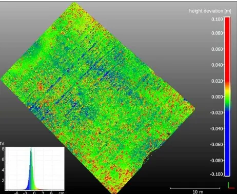
Figure 4 exemplary displays the complexity of the discrepancies between both high resolution topographic datasets. At local ridges and depressions high point deviations are obvious, potentially due to shadow and edge effects evolving from the TLS data. In locally smooth areas UAV and TLS data reveal higher accordance. Furthermore, systematic error patterns from the TLS point clouds are visible as point differences circuiting each SP. Blunders or large deviations are mainly due to local solely partly filtered vegetation spots, which are differently captured by UAV photogrammetry and TLS.
Figure 4: Calculated height deviation between TLS point cloud and UAV mesh (see also Tbl. 3). Point deviations exceeding ±10 cm are excluded from illustration due to blunders. TLS points above and below UAV mesh are red and blue, respectively.
During all field campaigns, TLS point clouds are about 1 cm lower than the UAV DEMs as highlighted in Table 3. However, this consistent deviation is not relevant due to the multi-temporal focus of this study, concentrating on relative data assessment for change detection. Furthermore, this error is partly corrected during data co-registration with ICP (Fig. 6). Highest data shifts are observable during the last field campaign (Tbl. 3), which might be due to the lower SP density (solely 6 instead of 8 as in the first two campaigns) resulting in an increase of the relative significance of errors that increase with increasing distance from the TLS device.
Highest standard deviation of TLS points to UAV mesh differences is measured during the first field campaign, which also depicts the DEM with the highest surface roughness, highlighting the potential consequence of edge and shadow effects. During the last field campaign, standard deviation is lowest, which might be the effect of decreasing surface roughness after prolonged submission to earth surface processes or the consequence of increased error smoothing of decreasing point densities (as demonstrated by Prosdocimi et al., 2015) compared to very high point densities during the first two campaigns.
mean standard deviation
17.09.2013 -8.9 mm 13.2 mm
01.11.2013 -9.8 mm 10.2 mm
14.02.2014 -10.9 mm 9.2 mm
Table 3. Difference between TLS points and UAV mesh.
3.2 Correction of systematic TLS error
The TLS point clouds of each SP reveal a sinusoidal deviation with maximum amplitude at a distance to the scanning device of about 7 m (Fig. 5). This instrument-specific systematic TLS error is eliminated corresponding to Eltner & Baumgart (2015), who use a reference plot of superior accuracy to derive a lookup table for the TLS correction. However, correction of the TLS data solely causes a minimal increase of the accuracy (Fig. 6.), which might be due to the generally high noise level of the yet unfiltered point cloud partly masking the systematic error. Besides the systematic errors, a comparison of the TLS point clouds of each SP to the UAV DEM further reveals a consistent shift of each TLS surface model, also visible in Figure 5.
Figure 5: Systematic error of TLS compared to UAV data (14.02.2014). a) Point deviations between surface mesh from UAV photogrammetry and uncorrected (upper image) and corrected (lower image) TLS point cloud of SP 1, b) averaged point deviations of all SPs.
3.3 UAV and TLS data co-registration
To account for the systematic shifts of the TLS data, co-registration with ICP caused significant improvement of the UAV and TLS data alignment (Fig. 6).
Figure 6. Result of TLS correction and co-registration of UAV and TLS data. SP-UAV-1: point deviations between UAV mesh and point clouds of individual SPs, SP-UAV-2: as SP-UAV-1 but TLS error corrected, SP-UAV-3: as SP-UAV-2 but TLS co-registered to UAV data, SP-SPs: as SP-UAV but comparison between SP and remaining SPs.
Different possible causes of the unfavourable TLS registration, besides the weak referencing geometry, are discussed in Eltner & Baumgart (2015), which are in short; difficulties to fit the retro-reflective cylinders, (device-intern) signal intensity manipulation, and increasing incidence angles with according difficulties of correct distance assignment in increasing footprints.
All SPs are compared to the UAV DEMs revealing a decrease of the mean and slight decrease of the standard deviation of the point differences (Fig. 6). The SPs were also compared solely amongst each other to guarantee a second method independent performance value, which confirms the improvement of data alignment due to the ICP approach.
3.4 UAV and TLS data combination
In this study, the thresholds have been defined as followed to derive data filtering with good results:
- The maximum distance between vegetation classified TLS point and the point from UAV photogrammetry amounts to 5 mm.
- The maximum incidence angle is set to 65°, corresponding to studies from Lichti (2007) and Soudarissanane et al. (2011), who detect a significant increase of outliers beyond this angle.
- The maximum footprint is defined at a size of 2.5 cm. - And the roughness per footprint has to be above 7 mm to be
excluded from the final point cloud fusion.
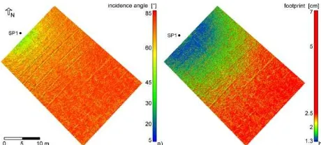
Due to the unfavourable perspective of the scanning device predominantly TLS points are excluded from the final digital soil surface model. This circumstance is also indicated by Fig. 7 because footprint and incidence angle increase quickly. The number of points of the TLS data decreases about 75%. Mainly points in close range to the SP are kept.
3.4.1 Considering data acquisition schemes: In this study, already in close proximities to the SPs unfavourable data acquisition scheme of TLS results in high incidence angles and footprints (Fig. 7). The opportunity to calculate the scan geometry with such high resolution is solely possible due to the availability of UAV DEMs with similar areal coverage. In studies with less data overlap, the estimates of TLS footprint and incidence angle will need stronger approximation because in these circumstances the reference surface for the retrieval of the scan geometry is more difficult to establish, e.g. the TLS data itself as a strongly smoothed surface representation or other less resolved data such as total station measurements.
Figure 7: Illustration of consequences of unfavourable scan geometry, i.e. fast decrease of a) incidence angle and b) footprint with increasing distance from the scanning device (Example from SP1 of the field campaign 14.02.2014).
3.4.2 Considering surface properties: The differing per-spectives of the different data acquisition methods onto the
points or at edges (Fig. 8). Roughness calculation allows for highlighting these locations. Thereby, isotropic roughness is calculated using a specific kernel size (here 9 cm), whose setting should be kept in mind because derived roughness parameters for soil surfaces are scale-dependent (e.g. Haubrock et al., 2009). Furthermore, anisotropic roughness is measured in this study, realised by consideration of height values within the footprint, which is oriented and distorted corresponding to the viewing direction of the scanning device. This roughness parameter reveals the selective relevance of local ridges and crests, and thus connected features, in regard to the SP in particular, which are not as clearly displayed with the isotropic roughness. Furthermore, the significance of the distance to the scanning device due to increasing footprints is also considered with the roughness per footprint value.
Figure 8: Importance of isotropic and anisotropic roughness as well as distance to scanning device for TLS point quality (field campaign 14.02.2014). a) hill-shaded UAV DEM, b) isotropic roughness, c) TLS point deviations to UAV DEM from SP1, d) roughness per footprint from SP1, e) TLS point deviations to UAV DEM from SP3, f) roughness per footprint from SP3.
The introduced approach to consider the surface properties as well as the data acquisition scheme before data merging from different sources is also transferable to other applications than soil erosion studies at field plots, e.g. in the case of gullys with overhangs captured with aerial and terrestrial images (e.g. Stöcker et al., 2015). Furthermore, the corresponding evaluation of each point performance can be extended in yet another stage considering the point quality with an according weight, e.g. to perform data smoothing with a weighted MLS. These point weights are also exploitable in regard to the estimation of level of detections, which especially consider local factors such as roughness, whose importance for geomorphic change detection has been demonstrated by Wheaton et al. (2010).
3.5 Multi-temporal changes
Regarding the complexity of soil topography, a constant decrease of the isotropic roughness parameter is detected over one season. It drops from 7 ± 4 mm in the first field campaign to 5 ± 3 mm and finally 3 ± 3 mm in the last campaign. Thus, the influence of rain drop impacts becomes obvious.
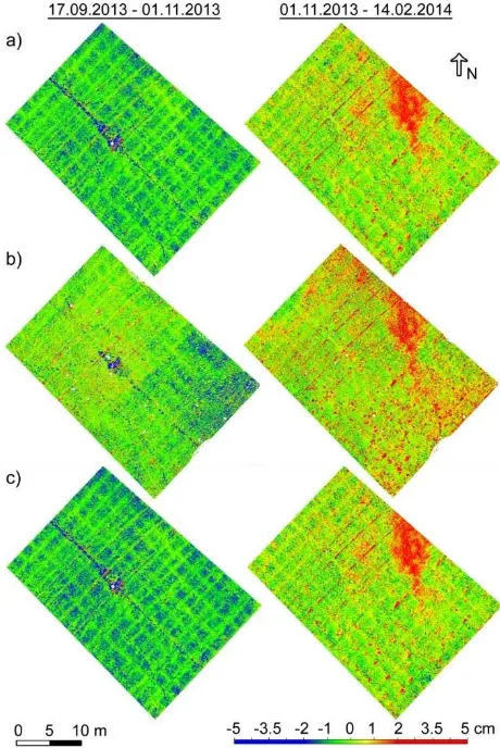
Change detection is performed between UAV data solely, TLS data solely, and fused UAV and TLS data, revealing the potential for more detailed surface description by the UAV DEMs compared to the TLS point clouds, which show higher data noise (Fig. 9), although TLS data has been post-processed according to Eltner & Baumgart (2015). Nevertheless, multi-temporal changes are consistent between both data sources in regard to magnitude and local depiction of height changes. Generally, local surface changes are obvious. In particular, the reappearance of former tractor tracks, during the period between the first and second field campaign, is interesting. They are assumed to occur due to less consolidation of the soil within the tracks after the tillage because the soil is already compacted in these locations. Furthermore, disconnected surface change patterns are visible, especially during the second study period between the second and last field campaign, i.e. the filling of local ridges resulting from cross-slope ploughing and the appearance of an alluvial fan with unknown sediment source from outside the field plot.
Figure 9: Multi-temporal surface changes. a) only considering UAV data, b) only considering TLS data, c) fused TLS and UAV data.
4. CONCLUSIONS
The capability of the introduced approach for a synergetic fusion of TLS and UAV data persists in the selective
combination of the point clouds in regard to scan geometry and surface roughness. Thus, in a further step weighted merging, corresponding to the data acquisition scheme as well as the surface properties, of datasets from different sources would be mandatory. However, more suitable data is needed because this study reveals the restricted adaptability of TLS for soil erosion studies at field plots, besides its eligibility for vegetation filtering and reliable error assessment. Future tests with comparable datasets in regard to the network of data capturing and surface interaction are necessary.
ACKNOWLEDGEMENTS
We thank the German Research Foundation (DFG) for funding this project (MA 2504/15-1). Furthermore, we are grateful for fruitful discussions with Pierre Karrasch and Frank Liebold. The data has been processed with Pix4Dmapper by Pix4D.
REFERENCES
Abellán, A., Jaboyedoff, M., Oppikofer, T., & Vilaplana, J. M., 2009. Detection of millimetric deformation using a terrestrial laser scanner: experiment and application to a rockfall event. Natural Hazards and Earth System Sciences, 9, pp. 365–372.
Barneveld, R. J., Seeger, M., & Maalen-Johansen, I., 2013. Assessment of terrestrial laser scanning technology for obtaining high-resolution DEMs of soils. Earth Surface Processes and Landforms, 38(1), pp. 90– 94.
Besl, P., & McKay, N., 1992. A Method for Registration of 3-D Shapes.
IEEE Transaction on Pattern Analysis and Machine Intelligence, pp. 14, 239–256.
Bracken, L. J., Turnbull, L., Wainwright, J., & Bogaart, P., 2015. Sediment connectivity: a framework for understanding sediment transfer at multiple scales. Earth Surface Processes and Landforms, 40, pp. 177–188.
Brodu, N., & Lague, D., 2012. 3D terrestrial lidar data classification of complex natural scenes using a multi-scale dimensionality criterion: Applications in geomorphology. ISPRS Journal of Photogrammetry and Remote Sensing, 68, pp. 121–134.
Cammeraat, L., 2004. Scale dependent thresholds in hydrological and erosion response of a semi-arid catchment in southeast Spain.
Agriculture, Ecosystems and Environment, 104(2), pp. 317–332.
Eltner, A., 2016. Photogrammetric techniques for across-scale soil erosion assessment. PhD thesis. Institute of Photogrammetry and Remote Sensing, TU Dresden. submitted.
Eltner, A., Kaiser, A., Carlos, C., Rock, G., Neugirg, F. & Abellan, A., 2015a. Image-based surface reconstruction in geomorphometry - merits, limits and developments of a promising tool for geoscientists. Earth Surface Dynamics Discussions, 3, pp. 1445-1508.
Eltner, A., Baumgart, P., Maas, H.-G., & Faust, D., 2015b. Multi-temporal UAV data for automatic measurement of rill and interrill erosion on loess soil. Earth Surface Processes and Landforms, 40(6), pp. 741–755.
Eltner, A., & Baumgart, P., 2015. Accuracy constraints of terrestrial Lidar data for soil erosion measurement: Application to a Mediterranean field plot. Geomorphology, 245, pp. 243–254.
Eltner, A., Mulsow, C., & Maas, H.-G., 2013. Quantitative measurement of soil erosion from TLS and UAV data. International Archives of the Photogrammetry, Remote Sensing and Spatial Information Sciences, XL(1/W2), pp. 119–124.
Eltner, A., & Schneider, D., 2015. Analysis of Different Methods for 3D Reconstruction of Natural Surfaces from Parallel-Axes UAV Images.
The Photogrammetric Record, 30(151), pp. 279–299.
Faust, D., & Schmidt, M., 2009. Soil erosion processes and sediment
fluxes in a Mediterranean marl landscape, Campiña de Cádiz, SW Spain. Zeitschrift für Geomorphologie, 53, pp. 247–265.
García-Ruiz, J., Nadal-Romero, E., Lana-Renault, N., & Beguería, S., 2013. Erosion in Mediterranean landscapes: Changes and future challenges. Geomorphology, 15, pp. 20–36.
Girardeau-Montaut, D., 2016. CloudCompare (version 2.6.2; GPL software), EDF RandD, Telecom ParisTech, available at: http://www.cloudcompare.org/, last access: 1 March 2016.
Haubrock, S.-N., Kuhnert, M., Chabrillat, S., Güntner, A., & Kaufmann, H., 2009. Spatiotemporal variations of soil surface roughness from in-situ laser scanning. Catena, 79, pp. 128–139. doi:10.1016/j.catena.2009.06.005
James, M. R., & Robson, S., 2014. Mitigating systematic error in topographic models derived from UAV and ground-based image networks. Earth Surface Processes and Landforms, 39, pp. 1413–1420.
Kraus, K., 2007. Photogrammetry: Geometry from Images and Laser Scans. 2nd edition, De Gruyter, Berlin, pp. 459.
Küng, O., Strecha, C., Beyeler, A., Zufferey, J.-C., Floreano, D., Fua, P., & Gervaix, F., 2012. the Accuracy of Automatic Photogrammetric Techniques on Ultra-Light Uav Imagery. International Archives of the Photogrammetry, Remote Sensing and Spatial Information Sciences, XXXVIII(1/C22), pp. 125–130.
Lichti, D. D., 2007. Error modelling, calibration and analysis of an AM–CW terrestrial laser scanner system. ISPRS Journal of Photogrammetry and Remote Sensing, 61(5), pp. 307–324.
Passalacqua, P., Belmont, P., Staley, D. M., Simley, J. D., Arrowsmith, J. R., Bode, C. A., Crosby, C., DeLong, S. B., Glenn, N. F., Kelly, S. A., Lague, D., Sangireddy, H., Schaffrath, K., Tarboton, D. G., Wasklewicz, T. & Wheaton, J. M., 2015. Analyzing high resolution topography for advancing the understanding of mass and energy transfer through landscapes: A review. Earth-Science Reviews, 148, pp.174-193.
Pesci, A., & Teza, G., 2008. Terrestrial laser scanner and retro-reflective targets: an experiment for anomalous effects investigation.
International Journal of Remote Sensing, 29, pp. 5749–5765.
Poesen, J., & Hooke, J. (1997). Erosion, flooding and channel management in Mediterranean environments of southern Europe.
Progress in Physical Geography, 21(2), pp. 157–199.
Prosdocimi, M., Calligaro, S., Sofia, G., Dalla Fontana, G., & Tarolli,
IEEE International Conference on Robotics and Automation, Shanghai, China.
Schürch, P., Densmore, A. L., Rosser, N. J., Lim, M., & McArdell, B. W., 2011. Detection of surface change in complex topography using terrestrial laser scanning: application to the Illgraben debris-flow channel. Earth Surface Processes and Landforms, 36, pp. 1847–1859.
Soudarissanane, S., Lindenbergh, R., Menenti, M., & Teunissen, P., 2011. Scanning geometry: Influencing factor on the quality of terrestrial laser scanning points. ISPRS Journal of Photogrammetry and Remote Sensing, 66(4), pp. 389–399.
Stöcker, C., Eltner, A. & Karrasch, P., 2015. Measuring gullies by synergetic application of UAV and close range photogrammetry — A case study from Andalusia, Spain. Catena, 132, pp. 1-11.
Vosselman, G. & Maas, H.-G., 2010. Airborne and Terrestrial Laser Scanning. Whittles Publishing, pp. 336.
Wheaton, J. M., Brasington, J., Darby, S. E. & Sear, D. A., 2010. Accounting for uncertainty in DEMs from repeat topographic surveys: improved sediment budgets. Earth Surface Processes and Landforms, 35, pp. 136-156.