NASA/TM–2009–215944
LAURA Users Manual: 5.2-43231
Alireza MazaheriAnalytical Mechanics Associates Inc., Hampton, Virginia Peter A. Gnoffo, Christopher O. Johnston, and Bil Kleb Langley Research Center, Hampton, Virginia
NASA STI Program . . . in Profile
Since its founding, NASA has been dedicated to the advancement of aeronautics and space science. The NASA scientific and technical information (STI) program plays a key part in helping NASA maintain this important role.
The NASA STI Program operates under the auspices of the Agency Chief Information Officer. It collects, organizes, provides for archiving, and disseminates NASA’s STI. The NASA STI Program provides access to the NASA Aeronautics and Space Database and its public interface, the NASA Technical Report Server, thus providing one of the largest collection of aeronautical and space science STI in the world. Results are published in both non-NASA channels and by NASA in the NASA STI Report Series, which includes the following report types: • TECHNICAL PUBLICATION. Reports of
completed research or a major significant phase of research that present the results of NASA programs and include extensive data or theoretical analysis. Includes compilations of significant scientific and technical data and information deemed to be of continuing reference value. NASA counterpart of peer-reviewed formal professional papers, but having less stringent limitations on manuscript length and extent of graphic presentations.
• TECHNICAL MEMORANDUM.
Scientific and technical findings that are preliminary or of specialized interest, e.g., quick release reports, working papers, and bibliographies that contain minimal annotation. Does not contain extensive analysis.
• CONTRACTOR REPORT. Scientific and technical findings by NASA-sponsored contractors and grantees.
• CONFERENCE PUBLICATION. Collected papers from scientific and technical conferences, symposia, seminars, or other meetings sponsored or
co-sponsored by NASA.
• SPECIAL PUBLICATION. Scientific, technical, or historical information from NASA programs, projects, and missions, often concerned with subjects having substantial public interest.
• TECHNICAL TRANSLATION. English-language translations of foreign scientific and technical material pertinent to NASA’s mission.
Specialized services also include creating custom thesauri, building customized databases, and organizing and publishing research results.
For more information about the NASA STI Program, see the following:
• Access the NASA STI program home page athttp://www.sti.nasa.gov
• E-mail your question via the Internet to [email protected]
• Fax your question to the NASA STI Help Desk at 443-757-5803
• Phone the NASA STI Help Desk at 443-757-5802
• Write to:
NASA STI Help Desk NASA Center for AeroSpace Information
7115 Standard Drive Hanover, MD 21076–1320
NASA/TM–2009–215944
LAURA Users Manual: 5.2-43231
Alireza MazaheriAnalytical Mechanics Associates Inc., Hampton, Virginia Peter A. Gnoffo, Christopher O. Johnston, and Bil Kleb Langley Research Center, Hampton, Virginia
National Aeronautics and Space Administration
The use of trademarks or names of manufacturers in this report is for accurate reporting and does not constitute an offical endorsement, either expressed or implied, of such products or manufacturers by the National Aeronautics and Space Administration.
Available from:
NASA Center for AeroSpace Information 7115 Standard Drive
Hanover, MD 21076-1320 443-757-5802
Abstract
This users manual provides in-depth information concerning installation and execution of Laura, version 5. Laura is a structured, multi-block, compu-tational aerothermodynamic simulation code. Version 5 represents a major refactoring of the original Fortran 77 Laura code toward a modular struc-ture afforded by Fortran 95. The refactoring improved usability and maintan-ability by eliminating the requirement for problem-dependent re-compilations, providing more intuitive distribution of functionality, and simplifying inter-faces required for multiphysics coupling. As a result, Laura now shares gas-physics modules, MPI modules, and other low-level modules with the Fun3D unstructured-grid code. In addition to internal refactoring, several new features and capabilities have been added, e.g., a GNU-standard instal-lation process, parallel load balancing, automatic trajectory point sequencing, free-energy minimization, and coupled ablation and flowfield radiation.
Contents
1 Introduction 5
2 New in This Version 6
3 Installation 8 3.1 Sequential installation . . . 8 3.2 MPI Installation . . . 9 4 Execution 10 5 Input Files 12 5.1 assign tasks . . . 12
5.1.1 Example 1: Multiple Blocks per CPU or Vice-versa . . 13
5.1.2 Example 2: Deactivating Grid Blocks . . . 14
5.2 laura.g . . . 14
5.3 laura bound data . . . 14
5.4 laura namelist data . . . 17
5.4.1 Ablation Flags . . . 17
5.4.2 Aerodynamic Coefficient Reference Quantities . . . 21
5.4.3 Farfield/Freestream Reference Quantities . . . 22
5.4.4 Grid Adaptation, Alignment, and Doubling Parameters 22 5.4.5 Grid File Description . . . 25
5.4.6 Initialization . . . 25
5.4.7 Molecular Transport Flags . . . 25
5.4.8 Numerical Parameters . . . 26
5.4.9 Radiation Flags . . . 28
5.4.10 Solid Surface Boundary Condition Flags . . . 28
5.4.11 Surface Recession Flags . . . 32
5.4.12 Thermochemical Nonequilibrium Flags . . . 33
5.4.13 Time Accurate Flags . . . 33
5.4.14 Trajectory Related Flags . . . 33
5.4.15 Turbulent Transport Models . . . 34
5.4.16 Venting Boundary Condition Flags . . . 34
5.5 tdata . . . 35
5.5.1 Perfect Gas . . . 35
5.5.2 Equilibrium Gas . . . 36
5.5.3 Mixture of Thermally Perfect Gases . . . 36
5.6 hara namelist data . . . 37
5.6.1 Specifying radiation mechanisms for atomic species . . 37
5.6.2 Specifying radiation mechanisms for molecular species . 38 5.6.3 Atomic line models . . . 40
5.6.5 Other flags . . . 42
5.7 kinetic data . . . 42
5.8 laura.rst . . . 44
5.9 laura.trn . . . 44
5.10 laura trajectory data . . . 44
5.11 laura vis data . . . 45
5.12 species thermo data . . . 46
5.13 species transp data . . . 48
5.14 species transp data 0 . . . 49
5.15 surface property data . . . 49
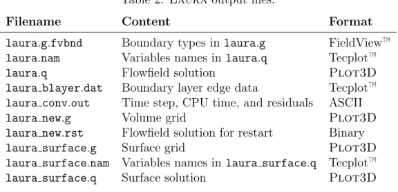
6 Output Files 52 6.1 laura.g.fvbnd . . . 53
6.2 laura.nam . . . 53
6.3 laura.q . . . 53
6.4 laura blayer.dat. . . 54
6.5 laura conv.out . . . 55
6.6 laura new.g . . . 55
6.7 laura new.rst. . . 55
6.8 laura surface.g . . . 56
6.9 laura surface.nam . . . 56
6.10 laura surface.q . . . 56
7 Laura Utilities 57 7.1 bounds . . . 57
7.2 coarsen . . . 57
7.3 convert bound data . . . 58
7.4 convert laura . . . 58
7.5 laura conv to tec . . . 58
7.6 laura stdout to tec. . . 58
7.7 make assign tasks . . . 59
7.8 self start . . . 59
7.9 shuffle laura . . . 59
8 Sample Cases 61 8.1 Sphere: 5-species Air, Thermo-chemical Nonequilibrium . . . . 61
8.2 Coupled radiation procedure . . . 66
8.3 Unspecified ablation procedure - Coupled . . . 67
8.4 Unspecified ablation procedure - Uncoupled . . . 69
A Migrating Cases from Prior Versions 72 B Additional Molecular Band Systems 75
C Trouble Shooting 77
C.1 Installation . . . 77
C.1.1 Unterminated Constant / Line Truncated . . . 77
C.2 Running . . . 77
C.2.1 NaNs . . . 78
C.2.2 Segmentation Faults . . . 78
1
Introduction
The users manual consists of seven sections. Section 2 gives an overview of new features, capabilities, and bug fixes. System requirements and installation are covered in Section 3, followed by code execution instructions in Section 4. Section 5 presents input files, their formats, and detailed information on their contents while Section 6 covers output files. Ancillary utilities are explained in Section 7, and the last section, Section 8, presents illustrative example cases.
2
New in This Version
Laurav5.2 offers several new enhancements and bug fixes since the previous released version, v5.1 [1]:
• Major Enhancements
– Automated radiation mechanism selection and streamlined user in-terface
– Added multi-processor per block capability for coupled radiation
• Minor Enhancements
– Extendedlaura blayer.dat to accommodate i and j surfaces
– Added Troubleshooting and Support sections
– To streamline the assignment of Plot3D function file variable names, Tecplot™ .namfiles are now produced instead of macros
– To facilitate plotting multiblock cases, a FieldView™ .fvbnd file is produced for volume data
– To play nice with *nix, codes now supply non-zero exit code upon failure
– To improve quality assurance, added technical debt build, unit test build with code coverage statistics, equilibrium air regression tests, and Shuttle Orbiter regression test
– To facilitate configuration management and code support, laura now emits version string via-Vor--versioncommand line options
• Bug Fixes
– Stop gracefully whentdata not found
– Multiprocessor run hangs for invalid namelist
– Equilibrium air data files not installed
– Intermittent failures of coupled ablation cases
– Load balancing for large numbers of processors
– Out of bound array in coupled ablation cases
– Logic error in algebraic turbulence models
– Pseudo-cell assignments across block boundaries
– Unrelated blocks exchanging information
– Undefined memory usage in radiation
– Out of bound array for radiation
– Initialization of ablation surface properties
– Full-fraction line implicit solves for certain multiblock grids
– Grid alignment for cases with axis singularity
– Partial-fraction line implicit for 3D cases
– Non-pivoting option for linear solver
For a complete revision history, please see theChangeLog file in the source distribution.
3
Installation
Laura requires a Fortran 95 compiler, and if parallel processing is desired, a Message Passing Interface (MPI) implementation.1 Some optional utilities
require Ruby.2 The installation and subsequent execution ofLauraassumes a Unix-like operating system or compatibility layer.3 After the code is unpacked
from the Laurarelease tarball,
% tar zxf laura-5.2-Z.tar.gz (unpack gzipped tarball) % cd laura-5.2-Z
where Z is a revision track number. Laura is installed via GNU build sys-tem,4 which entails executing a sequence of four commands: configure,make,
make check,5 and make install.6
3.1
Sequential installation
To configure, compile, test, and install a sequential version of Laurafor use with a single processor, first make a subdirectory oflaura-5.2-Z to store the configuration. For example,
% mkdir g95-seq % cd g95-seq
if using the g95 Fortran compiler;7 and then proceed with the typical GNU
build sequence,
% ../configure FC=g95 --prefix=$PWD % make
% make check % make install
Note that configure’s --prefix option specifies the root directory for in-stalling build artifacts—the default is /usr/local. In this example, it is set to the current working directory, g95-seq so executables will be installed in g95-seq/bin and data files will be copied to g95-seq/share/laura and g95-seq/share/physics modules directories.
To use Laura and associated utilities, set your search path to include $PWD/bin, e.g.,
setenv PATH ${PWD}/bin:$PATH (for csh) export PATH=${PWD}/bin:$PATH (for sh)
1For example, OpenMPI or MPICH.
2See ruby-lang.org.
3For non-Unix-like systems, compatibility layers are available from mingw.org (minimal)
and cygwin.com (maximal).
4See gnu.org/software/autoconf/.
5Themake checkcommand is optional. It will attempt to run small test cases. 6The
make install command may require administrator privileges depending on your installation location.
3.2
MPI Installation
An MPI-enabled installation (to allow multiple processors) is similar to the sequential installation except the configuration command has the--with-mpi option instead of theFC Fortran compiler variable, e.g.,
% ../configure --prefix=$PWD \
--with-mpi=/usr/local/pkgs/ompi_1.2.8-intel_11.0-028
Another difference is that an MPI-enable configuration will produce an exe-cutable named laura mpi instead of laura.
In either case, config.log contains a record of the configuration com-mand used, andconfigure’s --helpoption details all available configuration options.
4
Execution
The following steps outline a typical simulation cycle.8
Step 1. To start Laura, a Plot3D structured grid file is needed — see Section 5.2 on page 14 for more info. You may externally generate a grid using grid generation packages, such as Gridgen™, GridPro, and so forth, or useLaura’s interactive self startutility to generate a single-block structured grid for simple families of 2D, axisymmetric and 3D blunt bodies—see Section 7.8 on page 59.
Step 1a. Usingself start. To useself startto generate a single-block grid, simply execute this interactive utility, e.g.,
% self_start
and answer all the questions. After a successful execution, this utility will have generated the following files:
assign_tasks laura_bound_data
laura.g laura_namelist_data self_start.log
Examine the grid, laura.g, and proceed to Step 2.
Step 1b. External Grid Generation. Generate a single- or multi-block structured grid with the following rules:
i. Right-handed grid coordinates
ii. Longitudinal axis of the body aligned with thex-axis, oriented nose-to-tail
and write the grid coordinates into aPlot3Dfile,laura.g. Run the interactiveboundsutility (see Section 7.1 on page 57) and answer all the questions regarding the grid block topol-ogy:
% bounds
This utility will automatically generatelaura bound data, the connectivity file.
Step 2. If you did not useself start, createassign tasks (see Section 7.7 on page 59 for more info) and a laura namelist data file or copy the sample file from the [install prefix]/share/laura directory, where [install prefix] is the installation prefix specified when Laura was installed. Edit this file for your case—see Section 5.4 on page 17 for more detail.
8See Section 8 on page 61 for complete worked examples and Appendix A on page 72 for
Step 3. Create a tdata file (see Section 5.5 on page 35) to define the gas model condition for your specific simulation.9
Step 4. Run Laura,
% laura
or
% mpirun -np [#] laura_mpi
where # is the number of available processors. By the end of this step, the following files will have been generated:
laura_conv.out laura.g.fvbnd laura_new.g laura_new.rst laura_surface.q laura.q
laura_surface.nam laura.nam
Examine these files before proceeding to the next step.10
Step 5. Change irest flag in the laura namelist data (see Section 5.4 on page 17) from 0 to 1, and copy the new generated grid and solution files tolaura.g and laura.rstfiles; i.e.,
% cp laura_new.g laura.g % cp laura_new.rst laura.rst
Step 6. Repeat the previous two steps until iterative convergence.
9A sampletdatais available in the[install prefix]/share/physics modules
instal-lation directory. The other datafiles that reside in this directory, e.g., kinetics data,
species thermo data, species transp data, and species transp data 0, may also be copied and tailored to suit a different thermodynamic model, curve-fit data, or thermo-chemical reactions are needed. See Section 5.5 on page 35 for more detail.
5
Input Files
Nominally, Laura requires five input files as shown in the upper section of Table 1. Depending on the simulation requirements, however, other files may also be necessary and are shown in the second section of Table 1. All files are plain ASCII text unless otherwise noted.
Table 1: Laurainput files.
Filename Content
assign tasks Sweep and relaxation directions
laura.g* Plot3D grid
laura bound data Grid block face boundary conditions laura namelist data Simulation configuration
tdata Gas model
hara namelist data Radiation mechanisms
kinetic data Specie reactants and products laura.rst† Flowfield solution for restart laura.trn Transition location and length laura trajectory data Trajectory points
laura vis data Viscous term treatment species thermo data Specie thermodynamics species transp data Collision cross-sections
species transp data0 High-order collision cross-sections surface property data Thermochemical surface properties
*Fortran unformatted binary, 3-D whole, multiblock
Plot3D.
†Fortran unformatted binary.
The following subsections describe all input files in detail, beginning with the nominally required files and then proceeding alphabetically as shown in the table.
5.1
assign tasks
This file defines sweep and relaxation directions for each grid block. Each line, corresponding to each grid block, has six integers that are separated by at least one space. These integers correspond to nbk, mbk, mbr, lstrt, lstop, and mapcpu where
nbk
mbk
Sweep direction. The assigned value can be either1,2, or3, correspond-ing to i-,j-, or k-direction, respectively.
mbr
The line relaxation direction. Note: must be different than the sweep direction.
Options are:
0: Point-implicit, i.e., no line-relaxation 1: Line-implicit along i coordinate 2: Line-implicit along j coordinate 3: Line-implicit along k coordinate
lstrt
The starting grid index in the sweep direction. Typically1 .
lstop
The ending grid index in the sweep direction. Typically 0, which is shorthand for the maximum index.
mapcpu
CPU number for block nbk. Must be greater than zero. To run with a single processor, set this value to 1 for all grid blocks.
When starting a new simulation where the k-coordinate runs from the vehicle surface to the freestream boundary, sweeping in the k-coordinate and solving point-implicitly is recommended, i.e. mbk = 3 and mbr = 0. After the shock has stabilized, switch to streamwise sweeps and solve line-implicitly along the k-coordinate, i.e. mbk = 1 and mbr = 3.
5.1.1 Example 1: Multiple Blocks per CPU or Vice-versa
Suppose the grid has 2 blocks, but the number of available processors is not the same as the number of grid blocks. The user does not need to change any of the input files and can simply specify the number of processors available, e.g.,
% mpirun -np [#] laura_mpi
where # is the number of available processors. Laura automatically assigns processors to blocks such that each processor receives approximately same number of grid cells.
5.1.2 Example 2: Deactivating Grid Blocks
Suppose the grid has 50 blocks, but only blocks 20–25 need to be updated. In this case, assign tasks would contain only the active blocks, e.g.,
20 3 0 1 0 1 21 3 0 1 0 2 22 3 0 1 0 3 23 3 0 1 0 4 24 3 0 1 0 5 25 3 0 1 0 6 nbk mbk mbr lstrt lstop mapcpu
5.2
laura
.
g
This file is a multi-block, 3D-wholePlot3Dfile in Fortran unformatted binary format with double-precision reals. For convenience, here is a sample of the Fortran 95 code that Laurauses to read this file:
open ( 25, file='laura.g', form='unformatted' ) read(25) nblocks
...allocate i,j,kblk(nb) and grid memory...
read(25) (iblk(nb),jblk(nb),kblk(nb),nb=1,nblocks) do nb = 1, nblocks
ix1 = iblk(nb) ; jx1 = jblk(nb) ; kx1 = kblk(nb) ...allocate grid(nb)%x,y,z memory...
read(25) (((grid(nb)%x(i,j,k),i=1,ix1),j=1,jx1),k=1,kx1), & (((grid(nb)%y(i,j,k),i=1,ix1),j=1,jx1),k=1,kx1), & (((grid(nb)%z(i,j,k),i=1,ix1),j=1,jx1),k=1,kx1) end do
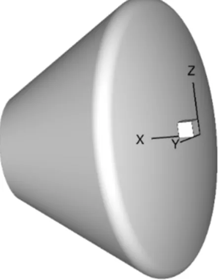
A file of this format, but named laura new.g,11 is generated by Laura at the
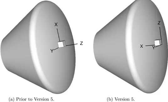
end of a successful run. This file is required and must have a right-handed coordinate system. Figure 1 shows the default laura coordinate orientation. Laura does not require a specific coordinate or grid orientation but the angle-of-attack definition is predefined — see Section 5.4.3 on page 22 for more info.
5.3
laura bound data
Grid block face boundary types are defined in laura bound data where each line corresponds to a grid block and contains six integers, one for each of the six faces: imin, imax, jmin, jmax, kmin, and kmax. Each integer specifies either
11When running a trajectory sequence, the file will be named
laura ####.gwhere ####
Figure 1: Default Lauracoordinate system orientation.
a physical boundary condition or block-to-block interfaces. An illustrative example is analyzed toward the end of this section.
This file is required and is generated automatically for grids created by Laura’sself startutility—see Section 7.8 on page 59. This file can also be created by using Laura’s interactive utility, bounds, by answering questions for each block.
Valid face types are as follows:
-9,...,0: Solid surface boundary. Up to ten different solid surface boundaries may be specified. Thermochemical properties of solid surfaces that are different than type 0, which are specified in laura namelist data, are defined in surface property datafile—see Section 5.15 on page 49.
1: Outflow boundary (extrapolation).
2: Symmetry boundary across y = constant.
3: Farfield/Freestream boundary.
4: Symmetry boundary across x = constant orz = constant.
5: Reflection boundary across j = 1 symmetry (valid for axi-symmetric and/or 2D grids).
6: Venting boundary. (See Section 5.4.16 on page 34 for more details.) 7: Reflection boundary across i face singularity with periodic j boundary.
>1000000: This seven digit boundary number defines block-to-block face connectiv-ity. The first digit is always1. The next three digits identifies the block number that is shared with the current block. The 5thdigit defines which i, j, or k face of the neighboring block is shared where 1 corresponds to
imin,2corresponds toimax, and so forth. The last two digits identify the
relation of the remaining two indices: The 6th digit can be either 1, 2,
3, or 4 where values of 1 or 3 mean the first index of the host face is in the same direction as the first or second index of the neighboring face, respectively, and values of 2 or 4 mean the adjoining indices are in the opposite direction. The last digit can be either a 1 or 2 and indicates whether the second indices of the host and neighboring faces are in the same direction or they are in the opposite direction, respectively.
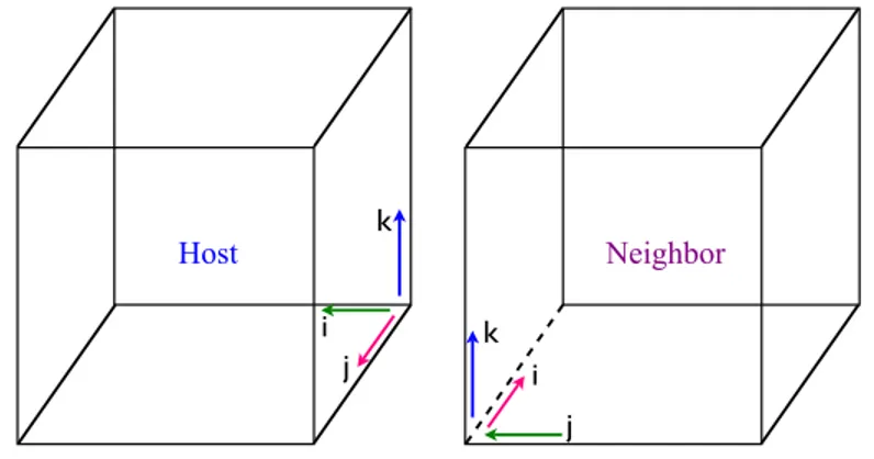
For example, consider a block with the followinglaura bound data bound-ary condition numbers:
1006421 1002111 2 1005121 0 3
The first integer, 1006421, shows that imin of this block is shared with jmax
(fifth digit) of block 6 (the first three digits after 1). The first and second indices of the host face are j and k, respectively. Because the j index is connected to i, the first and second indices of the neighboring face are i and
k, respectively, The 2 in the 6th digit shows that the j index of the host face
is in opposite direction of the i index of the neighboring face. The last digit, 1, indicates that k indices of the host and and neighboring faces are along the same direction. This configuration is illustrated in Figure 2.
i j k k i j Host Neighbor
Figure 2: Illustration used for block connectivity example.
The second and fourth boundary-type integers can be explained similarly. The third boundary-type integer (corresponding to the jmin face) specifies a
y-constant symmetry plane; the fifth boundary-type integer (corresponding to the kmin face) specifies is a solid-wall boundary condition; and the last digit
5.4
laura namelist data
Simulation configuration is specified throughlaura namelist data and is re-quired. This file is read as a Fortran 95 namelist and has the form,
&laura_namelist
velocity_ref = 5000.0 ! Free stream velocity, m/s density_ref = 0.023 ! reference density, kg/s tref = 250.0 ! Free stream temperature, K
alpha = 25.0 ! Angle-of-attack in xz plane, degrees [ variable = value ! Optional comment ]
/
where variable and their possible values are described in the following sec-tions, which are grouped according to farfield/freestream and aerodynamic coefficient reference quantities; thermochemical nonequilibrium flags; molec-ular transport flags; turbulent transport models flags; numerical parameters; grid adaptation, alignment, and doubling parameters; radiation and ablation flags; grid-file description; venting boundary condition flags; and solid sur-face boundary condition flags. Note that for all but the parameters shown in the above example, reasonable defaults have been chosen and only those parameters that differ from the defaults need to be specified.
Detailed description of parameters and/or flags with their units and default values is presented under each of the above categories. The order of these parameters is arbitrary but is given here alphabetically for better readability.
5.4.1 Ablation Flags
ablation option
An integer that specifies whether the pyrolysis ablation rate and wall temperature are computed in addition to the char ablation rate. This option only effects cases withbprime flag equal to 0 or 1.
Options are:
0: The pyrolysis ablation rate and wall temperature are computed, in addition to the char ablation rate, assuming steady-state ablation. 1: The pyrolysis ablation rate and wall temperature are held constant (they are set to the values present inablation from laura.m) while the char ablation rate is computed.
ablation verbose
A logical flag to print out developer focused info on convergence of ab-lation. Default: .true.
blowing model 0
Character indicator for ablation model specification. Default: ‘none’ Options are:
‘FIAT’
This ‘FIAT’12 option computes the blowing rate and surface tem-perature as a function of heating rate, pressure, and ablator ele-mental mass fractions. The user must specify the eleele-mental mass fractions for char and pyrolysis gas or default of 100% carbon will be employed.
‘none’
No ablation-flowfield coupling.
‘specified’
This option specifies a blowing or suction rate as a function of pres-sure (see mdot pressure 0). The user must specify the elemental mass fractions for pyrolysis gas or default of 100% carbon will be employed. Any specification for elemental mass fraction of char is ignored in this option.
‘equil char quasi steady’
This option solves the equilibrium surface ablation problem. The energy balance, elemental mass balance, and char equilibrium con-straint are solved to obtain the char ablation rate, wall temperature, and elemental composition at the surface. Along with the pressure from the normal momentum equation, these values define the equi-librium species composition at the wall. The user must specify the surface temperature type to be surface energy balance — see Section 5.4.10 on page 28 for more info.
Presently, this model does not include an in-depth material response computation, which would provide the pyrolysis ablation rate and conductive heat flux into the solid material. These two values are required for solving the previously mentioned surface equations. To approximate these values, the steady-state ablation assumption is made, which specifies that the pyrolysis ablation rate is propor-tional to the char ablation rate and the in-depth conduction is pro-portional to the enthalpy at the surface.
In the present framework of steady-state ablation, the ablation material is completely defined by CHONSi frac pyrolysis 0 (thus
12FIAT is a stand alone software and is needed if
blowing model 0=‘FIAT’. Request for access to FIAT can be made to NASA Ames Research Center.
CHONSi frac char 0 is ignored in this option). These are defined below. Note that the computed ablation rate is the sum of the py-rolysis and char components. (See Sections 8.3 on page 67 and 8.4 on page 69 for recommended procedure for an unspecified ablation computation.)
‘quasi steady’
This option specifies a quasi-steady ablation rate as a function of local pressure, heating rate, and temperature. The sublimation temperature and heat of ablation are specified by the user for a given ablator as a function of pressure. (See t sublimation 0 and h ablation 0.) If the surface temperature is less than the sub-limation temperature a zero blowing rate is defined. Otherwise the blowing rate is given by ˙m = q/∆Habl with appropriate
non-dimensionalization employed before use. The user must specify the elemental mass fractions for pyrolysis gas or default of 100% car-bon will be employed. Any specification for elemental mass frac-tion of char is ignored in this opfrac-tion. The user must specify the surface temperature type to be surface energy balance — see Section 5.4.10 on page 28 for more info.
bprime flag
An integer defining if the b-prime approach is applied. Applicable only forblowing model 0 = ‘equil char quasi steady’. See Section 5.4.1 on the preceding page for more details of its application. Default: 1 Options are:
0: Do not use bprime approach, and instead use a rigorous diffusion model. This option is consistent with the “Fully-Coupled” approach defined in Ref. [2].
1: Use b-prime approach. This option is consistent with the “Partially-Coupled” approach defined in Ref. [2].
2: Hold the ablation rate and wall temperature constant from the restart file, while applying the rigorous diffusion model (thus, the surface energy balance and char equilibrium constraint are not sat-isfied). This option is sometimes useful when transitioning from a bprime flag = 1 computation to a bprime flag = 0 computa-tion.
char density 0
Density of the char, kg/m3. Default: 256.29536, which is for the heritage
CHONSi frac char 0
This rank 1 vector of extent 5 sets elemental mass fraction of C, H, O, N, and Si species from char. Elemental mass fractions must be in this order and the sum of elemental mass fractions must equal1.0 . Default: CHONSi frac char 0 = 1.0, 0.0, 0.0, 0.0, 0.0
CHONSi frac pyrolysis 0
This rank 1 vector of extent 5 sets the elemental mass fractions of pyrol-ysis gas species, which are C, H, O, N, and Si. Elemental mass fractions must be in this order and the sum of elemental mass fractions must be 1. Default is Graphite:
CHONSi frac pyrolysis 0 = 1.0, 0.0, 0.0, 0.0, 0.0 compute mdot initial
An integer defining if the ablation rates are computed before the first flowfield iteration.
Options are:
0: Applies the ablation rates and wall temperatures present in the ablation from laura.m file.
1: Computes the ablation rates and wall temperatures before the first flowfield iteration.
freq wall
For bprime flag = 1, it is an integer defining frequency of update to ablation wall boundary conditions. For bprime flag = 0, it is an inte-ger defining frequency of update to the surface energy balance solution, which defines the wall temperature, whilenexchdefines the frequency of update to the remaining surface equations — see Section 5.4.8 on page 26 for more info on nexch. Default: 50
h ablation 0
A rank 1 vector of extent 3 used to compute the heat of ablation in MJ/kg for quasi steady blowing option as
h_ablation_0(1) + (h_ablation_0(2)) logpw
+ (h_ablation_0(3))(logpw)2
(1)
wherepw is the local pressure,in atmospheres. Example ∆Habl = 28.0−
1.375 logpw + 27.2(logpw)2. Default: 0.0
mdot pressure 0
A rank 1 vector of extent 2 is used to set the blowing or suction distri-bution defined as
mdot_pressure_0(1)+ (mdot_pressure_0(2)) p
ρ∞V∞2
where p is the local pressure, ρ∞ is the reference density, andV∞ is the reference velocity. Positive value produces blowing distribution, while negative value produces suction distribution. Default: 0.0
t sublimation 0
A rank 1 vector of extent 3 used to compute the sublimation temperature in degrees Kelvin for quasi steady blowing option as
t_sublimation_0(1) + (t_sublimation_0(2)) logpw
+ (t_sublimation_0(3))(logpw)2
(3)
wherepw is the local pressure,in atmospheres. ExampleTsub = 3797.0 +
342.0 logpw + 30.0(logpw)2. Default: 0.0
uncoupled ablation flag
An integer defining if an uncoupled ablation analysis is applied. The uncoupled ablation option is included to provide a baseline solution for the coupled ablation analysis. Default: 0
Options are:
0: Do not apply an uncoupled ablation analysis. It means that the coupled ablation analysis discussed in Section 8.3 on page 67 is applied.
1: Apply an uncoupled ablation analysis to a converged non-ablating flowfield. The procedure for applying the uncoupled ablation anal-ysis is discussed in Section 8.4 on page 69.
virgin density 0
Density of virgin material, kg/m3. Default: 544.627742, which is for the heritage AVCOAT.
5.4.2 Aerodynamic Coefficient Reference Quantities
bref
Yaw moment coefficient reference length, grid-units. Default: 1.0
cref
Pitching moment coefficient reference length, grid-units. Default: 1.0 sref
Reference area for aerodynamic coefficients, grid-units. Default: 1.0 xmc
ymc
y-coordinate of moment center, grid-units. Default: 0.0 zmc
z-coordinate of moment center, grid-units. Default: 0.0
5.4.3 Farfield/Freestream Reference Quantities
alpha
Angle-of-attack inxz plane, degrees, such that
u=cos(α)cos(yaw);v =−sin(yaw);w=sin(α)cos(yaw) (4) whereu, v, andw are velocities in x-, y-, and z-coordinate, respectively. Default: 0.0
density ref
Free stream density, kg/m3. Default: 0.001
rpm
Spin rate, RPM. This is applicable only to axisymmetric cases. Default: 0.0
tref
Free stream temperature, K. Default: 200.0
velocity ref
Free stream velocity, m/s. Default: 5000.0 yaw
Sideslip angle in xy plane, degrees. Default: 0.0
5.4.4 Grid Adaptation, Alignment, and Doubling Parameters
beta grd
This parameter controls grid points normal to the body (k-grid points) are controlled by the following grid stretching function:
ki∗ = 1−β β−1 β+1 kmax−ki kmax −1 β−1 β+1 kmax−ki kmax + 1 (5)
where ki∗ are new grid points. The beta_grd parameter defines the β
coefficient in equation 5. No stretching will be performed if β < 1. Recommended value is 1.15, if used. Default: 0.0
ep0 grd
Grid clustering around the shock is designed using the following function:
k∗∗
i =0ki∗
2
(1−k∗
i)(ki∗+fsh) +ki∗ (6)
whereki refers to normalized value andki∗ is defined by equation 5 on the
facing page. ep0 grd assigns the 0 coefficient in equation 6. Maximum
recommended value is 25/4, if used. Default: 0.0
kmax final
The target number of grid cells in the k-direction. Triggered by the global L2 error norm set by kmax error, cells along the k direction are increased by a factor of kmax factor until reaching kmax final. Any value less than the number ofk grid cells in laura.gfile will be ignored, i.e., no coarsening. This option requires all blocks to be active. Default: 0.0
kmax error
When the global L2 error norm reaches this value, the number of grid cells in the k direction increases by a factor of kmax factor until the maximum allowable grid cells, kmax final, is reached. This option re-quires all blocks to be active. Default: 0.01
fctrjmp
This parameter is used to detect bow shocks. Bow shock is first detected when the sensing parameter defined by jumpflagexceeds by this value, while searching from inflow boundary. Default: 1.05
frac line implicit
This positive parameter, which must be less than or equal 1, sets a fraction of the line-implicit direction that is assigned in assign tasks (see Section 5.1 on page 12). This parameter, which supersedes the given assignments in assign tasks, will be applied to all the active blocks. This parameter is recommended where there might be an instability issue such as across strong shocks. Default: 0.7
fsh
Fraction of arc length distance between body and inflow boundary where bow shock is captured. Default: 0.8
fstr
This parameter approximately defines fraction of k-cells in boundary layer region. Default: 0.75
jumpflag
An integer flag to select the sensing parameter to be used in detecting position of captured shock for grid adaption. Default: 2
Options are:
0: Redistributes grid points in k-direction for the target cell Reynolds number defined by re cell parameter, without changing the do-main boundary.
1: Selects pressure as the sensing parameter. 2: Selects density as the sensing parameter. 3: Selects temperature as the sensing parameter.
4: Scales the grid distance in the k-direction up by the value defined byfctrjmpparameter.
maxmoves
An integer number to assign maximum number of times that grid adap-tion is performed. The value of zero, however, can be used for unlimited number of times. Default: 0
max distance
This real number defines maximum distance from the body surface that grid outer boundary can be moved away by any one of the flags. This is often useful especially when adapting shock into wake, where the adapt-ing grid may become skewed due to presence of sharp gradients. This value defines the maximum length of the wake. Default: 1.0E+6
movegrd
An integer number for number of cycles between each grid alignment. A zero value disables any grid alignment. Default: 0
re cell
This value defines the target cell Reynolds number at the wall after a grid movement. Note : If the grid is moving radically Default: 0.1 Note: Use a higher value for re cell for the first grid alignment, if the grid movement causes radical changes in the grid.
The cell Reynolds number is defined as
Recell =ρc∆n/µ (7)
Here ρ is the flow density, c is the sound speed, ∆n is the cell height, and µis the flow viscosity.
5.4.5 Grid File Description
dimensionality
A string flag to select the dimensions of the problem. Default: ‘3D’. Available options are:
‘axisymmetric’
This option selects axisymmetric flow solution. This requires a domain with single-cell width in the j-direction.
‘2D’
This selects two-dimensional problem, which requires a domain with single-cell width in thej-direction.
‘3D’
This option solves three-dimensional problems. grid conversion factor
This parameter scales the grid to meter. One grid unit equalsgrid conversion factor meters. Default: 1
single precision grid
Logical flag: .true. if grid points in the laura.g file are stored as single precision values, otherwise double precision is assumed. Default: .false.
5.4.6 Initialization
init vel fctr
A real number between 0 and 1 to reduce the initial velocities u, v, w
within the domain to avoid creating a vacuum for wake flow problems, which may lead to an invalid solutions. The initial near zero velocity has also shown to ease up the formation of bow shock. Default: 0.01
5.4.7 Molecular Transport Flags
ivisc
An integer flag to engage viscous terms (inviscid=0/viscous=2). Default: 2
mass driven diff
A logical flag to engage binary diffusion driven by mass fraction gradient. Default: .false.
multi component diff
A logical flag to engage multi-component diffusion by Stefan-Maxwell equation sub-iterations. Default: .false.
mole driven diff
A logical flag to engage binary diffusion driven by mole fraction gradient. Default: .true.
navier stokes
A logical flag to select equation set for Thin-Layer Navier Stokes or Full Navier Stokes. The navier stokes = .false. may be used to select Thin-Layer Navier Stokes. Default: .false.
pressure diffusion
A logical flag to engage pressure diffusion term on Stefan-Maxwell ap-proximation. Default: .false.
schmidt number
A constant Schmidt number may be specified to calculate diffusivities. If the value is negative, diffusivities are computed directly from collision cross sections. Default: -1.0
prandtl number
A constant Prandtl number may be specified to calculate conductivi-ties. If the value is negative, conductivities are computed directly from collision cross sections. Default: -1.0
5.4.8 Numerical Parameters
cfl1
Initial value of CFL number. Default: 5.0 cfl2
Final value of CFL number. Default: 5.0 epsa
Eigenvalue limiting factor. Default: 0.3
hrs
The maximum total CPU time for simulation, hours. Default: 10
iramp
Number of cycles to ramp from cfl1 tocfl2. Default: 200
irest
An integer flag to start the simulation either using freestream values (irest = 0), or using the existing solution fromlaura.rstfile (irest = 1). Default 0
iterwrt
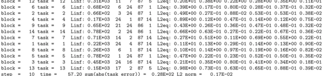
Number of cycles between saves of all output files—see Section 6 on page 52. Default: 200
jupdate
Number of cycles between jacobian updates. Default: 10 ncyc
Number of global iterations. Default: 1000
nexch
Number of cycles between exchange of data between processors and up-dating boundary conditions. Default: 2
nitfo
Number of cycles using 1st-order spatial accuracy. Default: 0
nordbc
Boundary condition calculation using 1st-order (nordbc = 1) or 2nd
-order (nordbc = 2) accuracy. Default: 1
ntran
Number of cycles between transport properties update. Default 1
rf inv
Inviscid relaxation factor. Default: 3.0 rf vis
Viscous relaxation factor. Default: 1.0 rf chem
Chemical source term reduction factor sometimes useful to ”ease in” simulations very close to equilibrium. This factor, which must be greater than 1.0 when it is used, changes the answers and must ultimately equal 1.0 in the final simulation. Default: 1.0
rmstol
A real number to stop the iterations after L2 norm residual reaches this value. Default: 1.0E-10
sub iterations
An integer number to control multiple passes through the linear solver, which has been found to increase robustness for some high energy appli-cations. Default: 1
5.4.9 Radiation Flags
radiation
A logical flag to enable coupling between radiation equation(s) and flow equations. See Section 8.2 on page 66 for coupled radiation procedure. Default: .false.
radiation input only
A logical flag to enable creation of input file hara out.m to compute radiation outside of Laurawhenradiationis.false.Default: .false.
maxrad
An integer number to assign maximum number of calls to radiation in-terface. The value of zero can be used for unlimited number of times. Default: 0
nrad
Number of iterations between calls to Hara. Default: 3000 iinc rad, jinc rad
Increment between i and j lines, respectively at which radiation profile is computed. Interim lines are interpolated. Default: 3
frac rad new
Relaxation factor on radiation. ∇(qrad) =f rac rad new∇(qrad)n+ (1−
f rac rad new)∇(qrad)n−1. Default: 1.0
absorptivity
Fraction of incident radiative energy absorbed by the wall. Affects sur-face energy balance and computation of radiative equilibrium wall tem-perature. Default: 1.0
tw rad flag
An integer flag to engage Tauber-Wakefield approximation for radiation cooling on surface-energy balance (on=1/off=0). Default: 0
5.4.10 Solid Surface Boundary Condition Flags
catalysis model 0
A character identifier for selecting catalysis model for surface type 0 (see Section 5.3 on page 14). This flag is good only for multi-species reacting gases and will be ignored for single-specie gas models. The catalysis model name must be surrounded by quotation marks, e.g.,‘ ’. Default: ‘super-catalytic’
‘CCAT-ACC’
This option uses the following surface catalytic coefficients [3] for catalyzing atomic oxygen and nitrogen to molecular oxygen and nitrogen, respectively. γO = 13.5e−8350/Tw∗ T∗ w ≤1359.0 K 5.0×10⁻⁸e18023/Tw∗ T∗ w >1359.0 K (8) γN = 4.0e−7625/Tw∗ T∗ w ≤1475.0 K 6.2×10⁻⁶e12100/Tw∗ T∗ w >1475.0K (9) whereTw∗ is calculated as Tw∗ =
min( max(1255.0, Tw), 1659.0) forγO
min( max(1255.0, Tw), 1900.0) forγN
(10)
‘CSiC’
This option uses the following surface catalytic coefficients [3] for catalyzing atomic oxygen and nitrogen to molecular oxygen and nitrogen, respectively. γO = 6.415×10⁻⁴e3498.4/T ∗ w (11) γN = 3.993×10⁻⁴e4402/T ∗ w (12) whereTw∗ is given as Tw∗ = min( max(1100.0, Tw), 1920.0) (13) ‘CSiC-SNECMA’
This option uses the following surface catalytic coefficients [3] for catalyzing atomic oxygen and nitrogen to molecular oxygen and nitrogen, respectively. γO=γN = 9.593×10⁻⁵e7002.9/T ∗ w (14) whereTw∗ is given as Tw∗ = min( max(1350.0, Tw), 1920.0) (15) ‘equilibrium-catalytic’
This option sets species concentrations to equilibrium values at wall pressure and temperature based on elemental mass fractions in the cell above the solid surface boundary.
‘fully-catalytic’
This option assumes that all the atomic and ionized oxygen, nitro-gen, carbon, and so forth catalyzes to molecular oxynitro-gen, nitronitro-gen, carbon, and so on, respectively; i.e.,
γO =γN =γC =...= 1 (16)
‘non-catalytic’
This option assumes that no atomic or ionized oxygen, nitrogen, carbon, and so forth catalyzes to molecular oxygen, nitrogen, car-bon, and so on, respectively; i.e.,
γO =γN =γC =...= 0 (17)
‘RCC-LVP’
This option uses the following surface catalytic coefficients [3] for catalyzing atomic oxygen and nitrogen to molecular oxygen and nitrogen, respectively. γO = 7.5e−8283/Tw∗ T∗ w ≤1499.0 K 2.5×10⁻⁷e17533/Tw∗ T∗ w >1499.0 K (18) γN = 6.0×10⁻²e−2605/Tw∗ T∗ w ≤1529.0K 1.5×10⁻⁵e10080/Tw∗ T∗ w >1529.0 K (19) whereTw∗ is calculated as Tw∗ =
min( max(1255.0, Tw), 1799.0) forγO
min( max(1255.0, Tw), 1954.0) forγN
(20)
‘Scott-RCG’
This option uses the following surface catalytic coefficients [4] for catalyzing atomic oxygen and nitrogen to molecular oxygen and nitrogen, respectively.
γO= 16.0e−10271/Tw 1400 ≤Tw ≤1650 (21)
γN = 7.14×10⁻²e−2219.0/Tw 1090≤Tw ≤1670 (22)
The same equations will be used even if the wall temperature, Tw,
is out of the specified range, in which case a warning will be issued to thestdout.
‘Stewart-RCG’
This option uses the following surface catalytic coefficients [3] for catalyzing atomic oxygen and nitrogen to molecular oxygen and
nitrogen, respectively. γO = 5.0×10⁻³e−400/Tw T w ≤502 1.6×10⁻⁴e1326/Tw 502< T w ≤978 5.2e−8835/Tw 978< T w ≤1617 39×10−9e21410/Tw 1617< T w (23) γN = 5.0×10⁻⁴ Tw ≤465 2.0×10⁻⁵e1500/Tw 465< T w ≤905 10.0e−10360/Tw 905< T w ≤1575 6.2×10⁻⁶e12100/Tw 1575< T w (24) ‘super-catalytic’
This option sets the species mass fractions to free stream values as defined intdata—see Section 5.5 on page 35.
‘Zoby-RCG’
This option uses the following surface catalytic coefficients [5] for catalyzing atomic oxygen and nitrogen to molecular oxygen and nitrogen, respectively.
γO = 9.41×10⁻³e−658.9/Tw 900≤Tw ≤1500 (25)
γN = 7.14×10⁻²e−2219.0/Tw 1090≤Tw ≤1670 (26)
The same equations will be used even if the wall temperature, Tw,
is out of the specified range, in which case a warning will be issued to the screen.
emiss a 0, emiss b 0, emiss c 0, emiss d 0
Real number values to calculate emissivity, , for solid surface boundary type (see Section 5.3 on page 14) from the following equation:
=a+bTw+cTw2 +dTw3 (27)
whereTw is the surface temperature. Values for a,b,c, and d are
de-fined byemiss a 0, emiss b 0, emiss c 0, and emiss d 0, respectively. Default: emiss a 0=0.89,emiss b 0=0.0,emiss c 0=0.0,emiss d 0=0.0 ept
Under-relaxation parameter for radiative equilibrium wall temperature:
qi,jn+1 = (1−eptqi,jn) +eptqi,jn+1 (28) wherendenotes iteration level,qi,jn+1is the most recent value of convective heat flux, qi,j, qi,jn is the value of convective heat flux from the previous
iteration as adjusted by previous application of this formula, andqni,j+1 is the newly adjusted value for convective heat flux at the n+ 1 iteration level. Default: 0.01
surface temperature type 0
Character identifier for surface temperature model selection. Default: ‘constant’
Options are:
‘adiabatic’
Surface temperature will be such that there is no heat transfer be-tween the surface and the gas adjacent to the surface.
‘constant’
The surface temperature stays constant as given bytwall bcvalue.
‘radiative equilibrium’
The surface temperature is calculated so that the heat flux to the wall,qw, is in equilibrium with radiation heat flux:
qw =σTw4 (29)
where σ is the Stefan-Boltzmann constant, and is the surface emissivity defined by emiss a 0, emiss b 0, emiss c 0, emiss d 0 values.
‘surface energy balance’
This option is required for ablating surfaces to compute surface temperature as a function of the surface energy balance and the relevant surface chemistry kinetics.
surface group name 0
Character descriptor for surfaces with solid surface boundary types (see Section 5.3 on page 14). Any character can be specified to group solid surface boundaries. Default: ‘default surface 0’
twall bc
Initial wall temperature for solid surface boundaries, K. (See Section 5.3 on page 14.) The wall temperature stays constant as specified by this pa-rameter ifsurface temperature type 0 = ‘constant’. Default: 500.0
5.4.11 Surface Recession Flags
shape change
A logical flag engaging the geometry shape change due to ablation. De-fault : .false. A trajectory file is required if shape change=.true. — see Section 5.10 on page 44.
5.4.12 Thermochemical Nonequilibrium Flags
chem flag
An integer flag to engage chemical source term for non-equilibrium flow (on=1/off=0). Default: 0
therm flag
An integer flag to engage thermal source term for non-equilibrium flow (on=1/off=0). Default: 0
5.4.13 Time Accurate Flags
itime
An integer flag to engage (itime = 1) or disable (itime = 0) time ac-curate simulation. Default: 0
subiters
An integer number to specify number of iterations between each time step for time-accurate simulations. Default: 10
5.4.14 Trajectory Related Flags
trajectory data point
Pickup simulation from this line in the file laura trajectory data. Default: 0 if laura trajectory datais not present.
Default: 1 if laura trajectory datais present.
Note that the reference quantities are defined consistently across the trajectory using the values supplied in namelist above. The reference quantities are NOT reset according to the time varying free stream con-ditions. Consequently, dimensionless values of density and velocity in free stream will not generally equal 1. Dimensionless values of total en-thalpy in free stream will not equal 0.5 which may impact post-processing tools that are key on a specific number for total enthalpy to detect the boundary-layer edge.
The algorithm is most efficient if the restart solution is converged (or nearly converged so that line-implicit relaxation may be applied) at free stream conditions equal to the reference quantities inlaura namelist data. If one wishes to pickup a computation for trajectory data point >1 then it is best to start at the converged restart file for the previous trajectory point. Restart files and post processing files for each tra-jectory point have the tratra-jectory point number included as part of the root name. Thus if one wants to pickup at trajectory point 12 one
should copylaura 0011.rsttolaura.rstand (if grid is being updated) laura 0011.gtolaura.g. This advice is offered because restart solutions are converted according to the ratio of density and velocity between ad-jacent trajectory points to bring interior initial conditions closer to the new inflow boundary conditions.
5.4.15 Turbulent Transport Models
prandtl turb
Turbulent Prandtl number. Default: 0.9 schmidt turb
Turbulent Schmidt number. Default: 0.9 turb int inf
Farfield turbulent intensity non-dimensionalized by square of the refer-ence velocity. Default: 0.001
turb model type
An integer flag to select turbulence modeling. Default: 0 Options are:
-1: Baldwin-Lomax algebraic turbulence model. [6] -2: Cebeci-Smith algebraic turbulence model. [6]
0: Laminar flow, i.e., no turbulence model. turb vis ratio inf
Farfield ratio of turbulent to laminar viscosity. Default: 0.01
xtr
Transition location along x-axis in grid units. Default: 0.0
5.4.16 Venting Boundary Condition Flags
vacuum pressure coefficient
This parameter, which is in N/m2 sets the pressure coefficient behind
type 6 boundaries (see Section 5.3 on page 14), which forces flow out of the domain. This coefficient is defined as
vacuum_pressure_coefficient= p0−p∞
2 . (30)
wherep0 is back pressure where the gas is venting out, andp∞ is farfield pressure. Default: 0.0
vacuum pressure factor
Factor on pressure across type 6 boundary to force flow out of domain.
vacuum_pressure_factor= p0
p1
, (31)
where p1 is the pressure just before the gas vents out. Default: 0.01
5.5
tdata
The gas model is defined in this file. It contains a list of key words, sometimes followed by numeric values, which identify components of the gas model. One or more spaces must be present between keyword and values when appearing on the same line. Spaces may appear to the left or right of any key word. The first line of the file must not be blank, however.
The following subsections describe available gas model options.
5.5.1 Perfect Gas
The perfect-gas option is engaged with either of the following keywords: perfect gas, PERFECT GAS,Perfect Gas, or Perfect gas.
If no further data is provided in this file, this single line tdata file will assume the following parameter values in SI units:
gamma = 1.4 mol_wt = 28.8
suther1 = 0.1458205E-05 suther2 = 110.333333 prand = 0.72
Here, gamma is the gas specific heat ratio, mol wtis the gas molecular weight, prand is the gas Prandtl number, andsuther1 andsuther2 are the first and second Sutherland’s viscosity coefficients, s1 and s2, respectively, defined as
µ=s1 T3/2 T +s2
(32)
These values can be modified and explicitly defined in the tdata by the keyword &species propertiesin the second line followed by the gas param-eters and / at the last line of the file. For example,
perfect_gas &species_properties gamma = 1.4 mol_wt = 28.0 suther1 = 0.1E-05 suther2 = 110.3 prand = 0.7 /
5.5.2 Equilibrium Gas
To engage the Tannehill curve fits for thermodynamic and transport properties of equilibrium air [7], the following keyword should be used in the first line of the tdata file: equilibrium air t. No additional inputs or files are required to engage the Tannehill option for equilibrium air.
To use a table look-up capability for equilibrium gases [8], the following keyword should be placed in thetdatafile, instead: equilibrium air r. Note that this option still uses the Tannehill transport properties.
5.5.3 Mixture of Thermally Perfect Gases
If the gas is a mixture of thermally perfect gases and multi-species transport solution is desired the species names followed by their mass fractions must be provided in the tdata file. Thermal state of the gas may be defined as the first entry by either of the following flags:
one
This flag assumes that all the species are thermally in equilibrium state. That is translational temperature, T, and vibrational temperature, Tv
are equal. This is known as one-temperature, 1-T, model.
two
This flag assumes that energy distribution in the translational and rota-tional modes of heavy particles (not electrons) are equilibrated at trans-lational temperature, T, and all other energy modes (vibrational, elec-tronic, electron translational) are equilibrated at vibrational tempera-ture, Tv. This is known as two-temperature, 2-T, model.
FEM
This option, called Free-Energy Minimization, causes the species conti-nuity equations to be replaced with elemental conticonti-nuity equations and equilibrium relations for remaining species.
One temperature model is assumed if thermal state of the gas is not provided in the first line of thetdatafile. In this case, the first line must contain species information. Note, the first line must not be blank.
Subsequent file entries include species names and their mass fractions at freestream/farfield boundary. Only one specie per line is allowed. The species mass fraction at the boundary is defined in the same line as the species name separated by one or more spaces. If no value appears to the right of the species name then that species is assumed not to be present at the boundary but may be produced through chemical reactions elsewhere in the flowfield.
Example 1: 1-T, 5-species air model: In this example, only molecular oxygen and nitrogen are present on freestream/farfield boundary, but atomic nitrogen and oxygen and nitric oxide may be produced elsewhere in the flow field due to chemical reactions.
one N2 .767 N O2 .233 O NO
Example 2: 2-T, 11-species air model: In this example, the gas is as-sumed to be a mixture of 11 thermally perfect gases. A solution to a thermal non-equilibrium state of the gas is also desired (2-T model).
two N2 .767 N O2 .233 O NO O2+ O+ NO+
e-5.6
hara namelist data
This file controls the radiation models used by the Hara radiation mod-ule [9, 10]. It is optional for coupled radiation simulations. If it is not present, then the code automatically chooses the radiative mechanisms associated with species present in the flowfield (and have number densities greater than 1000 particles/cm2), and other options are set to the defaults listed in the following
section. For users not experienced in shock-layer radiation, it is recommended that thishara namelist datafile not be applied (meaning it is removed from the working directory), therefore allowing the radiative mechanisms to be au-tomatically chosen and the default model options applied.
5.6.1 Specifying radiation mechanisms for atomic species
The treatment of radiation resulting from atomic lines, atomic bound-free and free-free photoionization (referred to here as atomic continuum), and neg-ative ion continuum is available for atomic carbon, hydrogen, oxygen, and nitrogen. These mechanisms are specified through the following binary flags
(on=1/off=0). If any of these flags are not present in hara namelist data, then that flag is set to true only if the number density of the associated atomic specie is greater than 1000 particles/cm2 somewhere in the flowfield.
treat [?] lines
A binary flag to enable the treatment of atomic lines for specie [?], where [?] can be c, h, n, and o, for atomic carbon, hydrogen, nitrogen and oxygen, respectively.
treat [?] cont
A binary flag to enable the treatment of atomic bound-free and free-free continuum for specie [?], where [?] can be c, h, n, and o, for atomic carbon, hydrogen, nitrogen and oxygen, respectively.
treat [?] other
A binary flag to enable the treatment of the negative-ion continuum for specie[?], where[?]can be c, h, n, and o, for atomic carbon, hydrogen, nitrogen and oxygen, respectively.
5.6.2 Specifying radiation mechanisms for molecular species
The treatment of radiation resulting from numerous molecular band systems is available through the following binary flags (on=1/off=0). If any of these flags are not present in hara namelist data, then that flag is set to true only if the number density of the associated molecular specie is greater than 1000 particles/cm2 somewhere in the flowfield. Additional band systems are listed in Appendix B on page 75. These additional band systems are generally considered negligible relative to those listed in this section, and therefore for computational efficiency, they are not engaged by default. Definitions of each band system and the modeling data applied are discussed in Refs. [9, 11].
treat band c2 swan
A binary flag activating the C2 Swan band system.
treat band c2h
A binary flag activating the C2H band system.
treat band c3
A binary flag activating the C3 and Vacuum Ultra-Violet (VUV) band
systems.
treat band cn red
treat band cn violet
A binary flag activating the CN violet band system.
treat band co4p
A binary flag activating the CO 4+ band system.
treat band co bx
A binary flag activating the CO B-X band system.
treat band co cx
A binary flag activating the CO C-X band system.
treat band co ex
A binary flag activating the CO E-X band system.
treat band h2 lyman
A binary flag activating the H2 Lyman band system.
treat band h2 werner
A binary flag activating the H2 Werner band system.
treat band n2fp
A binary flag activating the N2 1+ band system.
treat band n2sp
A binary flag activating the N2 2+ band system.
treat band n2pfn
A binary flag activating the N+2 first-negative band system. treat band n2 bh1
A binary flag activating the N2 Birge-Hopfield I band system.
treat band n2 bh2
A binary flag activating the N2 Birge-Hopfield II band system.
treat band no beta
A binary flag activating the NO beta band system.
treat band no delta
A binary flag activating the NO delta band system.
treat band no epsilon
5.6.3 Atomic line models
There are various models available for atomic line radiation, one of which must be chosen for each specie that engages atomic line radiation (as specified using treat [?] lines). This choice of atomic line model is made using the following flags. The listed defaults are applied if the individual flag is not present in hara namelist data, or if hara namelist data is not present in the working directory. All model types in this category must be surrounded by a quotation marks, e.g. ‘ ’.
c atomic line model, h atomic line model
A character identifier for selecting the atomic line model for atomic car-bon or hydrogen. Presently, the only available option is the model com-piled in Ref. [11], which is referred to here as the Complete Line Model (CLM). Default : ‘clm’
n atomic line model, o atomic line model
A character identifier for selecting the atomic line model for atomic ni-trogen or oxygen. The available models are compiled and compared in Ref. [9], which is referred to here as the Complete Line Model (CLM). Default : ‘clm’ Available models are:
‘all multiplets’
This model treats all lines as grouped multiplets. This significantly reduces the number of lines treated as well as the computational expense. However, this grouped multiplet approximation will lead to errors for non-optically-thin conditions.
‘clm’
This model, which stands for Complete Line Model, applies the individual treatment of strong atomic lines while applying multiplet averages for weak lines. This is the recommended model.
5.6.4 Electronic state population models
These flags specify the model applied for predicting the electronic state popu-lations of atoms and molecules. The listed defaults are applied if the individual flag is not present in hara namelist data, or if hara namelist data is not present in the working directory. All model types in this category must be surrounded by a quotation marks, e.g. ‘ ’.
Atomic electronic states
The electronic state populations for atoms are required for computing atomic line and photoionization emission and absorption. The compilation and com-parison of the available models are presented in Ref. [10].
c electronic state, h electronic state
A character identifier for selecting the electronic state model for atomic carbon and hydrogen. Available models are (Default : ‘boltzmann’):
‘boltzmann’
Applies Boltzmann population of electronic states.
‘Gally 1st order LTNE’
Applies the Gally first-order local thermodynamic nonequilibrium method [13], which approximately accounts for the non-Boltzmann population of atomic states.
n electronic state, o electronic state
A character identifier for selecting the electronic state model for atomic nitrogen and oxygen. Available models are (Default : ‘CR’):
‘boltzmann’
Same as for c electronic state
‘Gally 1st order LTNE’
Same as for c electronic state
‘CR’
Applies the detailed Collisional Radiative (CR) model developed in Ref. [10].
‘AARC’
Applies the Approximate Atomic Collisional Radiative (AARC) model developed in Ref. [10]. This model is essentially a curve-fit based approximation of the CR model, which allows for improved computational efficiency with a slight loss in accuracy.
Molecular electronic states
The electronic state populations for molecules are required for computing molecular band emission and absorption. The compilation and comparison of the available models are presented in Refs. [10, 14].
molecular electronic state
A character identifier for selecting molecular electronic state for all molec-ular band systems. Available models are (Default : ‘CR’):
‘boltzmann’
‘CR’
Applies a detailed Collisional Radiative model considering both heavy-particle and electron impact transitions. Some molecular states are still assumed Boltzmann with this model because no data is presently available for the CR model.
5.6.5 Other flags
use triangles
A logical flag specifying whether optically-thin atomic lines are modeled as triangles to reduce computational time. This option has shown to result in a negligible loss of accuracy while greatly reducing the compu-tational time, [9] and is therefore recommended. Default : .true. Note: This flag is automatically set to.true.whenn oro atomic line model= ‘clm’ — see Section 5.6.3 on page 40.
use edge shift
A logical flag to engage the photoionization edge shift [9] for atomic bound-free radiation. (on=1/off=0). Default : .true.
5.7
kinetic data
This file defines possible chemical reactions and is optional. By default, kinetic datais read from[install-prefix]/share/physics modules, but if present in the local run directory, Laura will read reactions from the local file instead.13
Reactants and products can be any species defined in thespecies thermo data file—see Section 5.12 on page 46. A sample entry looks like this,
O2 + M <=> 2O + M 1 2.000e+21 -1.50 5.936e+04 2 teff1 = 2 3 exp1 = 0.7 4 t_eff_min = 1000. 5 t_eff_max = 50000. 6 C = 5.0 7 O = 5.0 8 N = 5.0 9 H = 5.0 10 Si = 5.0 11 e- = 0. 12
13The precise installation location is given by
Laura during startup. It can also be found on Unix-like systems from the executable itself by issuing the command
The first line specifies the reaction while line 2 provides three coefficients of an Arrhenius-like equation, Kf =cfT η ef fe −0/kTef f (33)
where cf is the pre-exponential factor, η is the power of temperature
depen-dence on the pre-exponential factor,0 is the Arrhenius activation energy, and k is the Boltzmann constant. The arrowheads in line 1 signify the allowed directionality of the reaction. The symbol => denotes forward reaction only while <=> denotes forward and backward rates are computed. The coeffi-cients in line 2 correspond to cf, η, and 0/k, respectively. For reactions with
a generic collision partner, M, such as this one, these coefficients correspond to Argon; and other collision partners and their efficiencies (multipliers ofcf)
are specified on lines following line 5 and 6, which give the valid temperature range for the reaction. The effective temperature, Tef f, is defined according
to a given integer number in line 3; Default: 2
teff1,teff2
Flag defining formula to compute the effective temperature Tef f for the
forward rate and backward rate, respectively. It is engaged for the case of thermal nonequilibrium. Options for teff are:
1: Tef f =Ttr
2: Tef f =Ttrexp1Tv1−exp1
3: Tef f =Tv
whereTtr andTv are translational and vibrational temperatures,
respec-tively. Default: 1
exp1
The exponent used to define the effective temperature when teff1 = 2 (forward rate) orteff2 = 2 (backward rate). See previous equations for teff options. Default: 0.7
t eff min
The minimum temperature forTef f to compute reaction rates to
circum-vent stiff source terms. Default: 1000.
t eff max
The maximum temperature for Tef f to compute reaction rates to