Design research in statistics education: On symbolizing and computer tools / A. Bakker – Utrecht: CD-β Press, Center for Science and Mathematics Education – (CD-β wetenschappelijke bibliotheek; nr. 50; 2004)
Dissertation Utrecht University. – With references. – With a summary. – Met een samenvatting in het Nederlands.
ISBN 90-73346-58-4
Subject headings: mathematics education, design research, technology, semiotics, history of statistics
Cover: Zuidam & Uithof, Utrecht Press: Wilco, Amersfoort
On symbolizing and computer tools
Ontwikkelingsonderzoek in het statistiekonderwijs
Over symboliseren en computertools
(met een samenvatting in het Nederlands)
PROEFSCHRIFT
TER VERKRIJGING VAN DE GRAAD VAN DOCTOR AAN DE UNIVERSITEIT UTRECHT,
OP GEZAG VAN DE RECTOR MAGNIFICUS PROF. DR. W. GISPEN INGEVOLGE HET BESLUIT VAN HET COLLEGE VOOR PROMOTIES
IN HET OPENBAAR TE VERDEDIGEN OP
MAANDAG 24 MEI 2004 DES MIDDAGS TE 14:30 UUR
door
Arthur Bakker
Prof. dr. K.P.E. Gravemeijer Faculteit Sociale Wetenschappen, Universiteit Utrecht
Faculteit Wiskunde en Informatica, Universiteit Utrecht
Prof. dr. G. Kanselaar Faculteit Sociale Wetenschappen, Universiteit Utrecht
Prof. dr. J. de Lange Faculteit Wiskunde en Informatica, Universiteit Utrecht
I have always enjoyed reading prefaces of dissertations because they often reveal something about the person behind the text and about the litany of people involved in the research.
Although I was unable to formulate it in this way as a youngster, I have always been intrigued by how people think and learn. At school I read histories of philosophy to see where ideas came from, I learned to play the violin (my mother being a violinist and music therapist), psychology sounded interesting, and artificial intelligence was ‘hot’. However, due to my father (a mathematics teacher) and the Mathematics and Pythagoras Olympiads, mathematics eventually caught my imagination as the purest form of human thinking. I chose to study mathematics, but its relations to other dis-ciplines such as philosophy, logic, history, and education continually demanded attention. After receiving a Master’s degree in mathematics, investigating the philo-sophical foundations of set theory proved rewarding, but this pursuit seemed some-how irrelevant to society. And while teaching secondary school mathematics felt very relevant, it was not my calling.
In 1998, I acquired a graduate position (onderzoeker in opleiding) at the Freudenthal Institute and mathematics education turned out to be the interdisciplinary mix I had been looking for without knowing it. This mix is reflected in my thesis: I studied the history of statistics to understand how statistical concepts evolved and to gain in-sights into promising ways to teach them. Conducting the design research required incorporating insights from educational science, psychology, mathematics and sta-tistics education, and practical experience as a teacher. Last, the semiotic analyses reflect my interest in the philosophy of language.
First, I would like to express my gratitude to Koeno Gravemeijer, who succeeded in raising the funds for this project from the Netherlands Organization for Scientific Research (NWO). He coached me along the route of becoming a researcher in math-ematics and statistics education. Gellof Kanselaar and Jan de Lange complemented the advisory team, each in their own helpful way. For more specialized topics I con-sulted experts who were forthcoming in their commentary on various chapters: Paul Cobb (Chapters 2, 4, and 8), Stephen Stigler (4), Cliff Konold (2, 4), and Michael Hoffmann (6, 8, 9). Thank you, Paul, Cliff, and Michael, for rewarding meetings and your hospitality as well. I also like to mention the inspiration I received from the Fo-rum for Statistical Reasoning, Thinking, and Literacy, chaired by Dani Ben-Zvi and Joan Garfield.
commu-like to thank two colleagues, Mieke Abels and Corine van den Boer, who also taught during the teaching experiments, and their students. Aad Goddijn and Martin Kindt were always willing to discuss mathematical and historical issues.
The ways in which I have been assisted are numerous. Petra van Loon, Harm Ber-gevoet, Carolien de Zwart, Sofie Goemans, and Yan Wei Zhou assisted during the teaching experiments by interviewing and videotaping. Han Hermsen taught me how to use Framemaker, the word processor with which this book has been made. Tanja Klooster, Ellen Hanepen, and Parul Slegers helped to transcribe students’ ut-terances. Anneleen Post, among others, helped me when Repetitive Strain Injury (or Carpal Tunnel Syndrome) hindered my work at the computer. Nathalie Kuijpers and Tim Muentzer corrected my English and Betty Heijman and Sylvia Eerhart assisted in the book’s publication. And of course I would like to thank Frans van Galen with whom I have shared my office all these years. Huub van Baar and Yolande Jansen supported me as friends and ushers (paranimfen). Thank you all!
1
Introduction . . . 1
1.1 Statistics education. . . 1
1.2 Design research . . . 3
1.3 Symbolizing . . . 3
1.4 Computer tools. . . 4
2
Background and research questions . . . 5
2.1 Realistic Mathematics Education (RME) . . . 5
2.2 Trends in statistics education research. . . 8
2.3 Nashville research with the Minitools . . . 17
2.4 Research questions. . . 34
3
Methodology and subjects . . . 37
3.1 Design research methodology . . . 37
3.2 Hypothetical learning trajectory (HLT) . . . 39
3.3 Phase 1: Preparation and design. . . 41
3.4 Phase 2: Teaching experiment . . . 42
3.5 Phase 3: Retrospective analysis . . . 45
3.6 Reliability and validity. . . 46
3.7 Overview of the teaching experiments and subjects . . . 47
4
A historical phenomenology . . . 51
4.1 Purpose. . . 51
4.2 Method . . . 52
4.3 Average . . . 53
4.4 Sampling . . . 61
4.5 Median . . . 65
4.6 Distribution . . . 74
4.7 Graphs . . . 80
5.1 Exploratory interviews . . . 92
5.2 Didactical phenomenology of distribution . . . 100
5.3 Didactical phenomenology of center, spread, and sampling . . . 104
5.4 Initial outline of a hypothetical learning trajectory . . . 109
6
Designing a hypothetical learning trajectory for grade 7 . . . 111
6.1 Outline of the hypothetical learning trajectory revisited . . . 111
6.2 Estimation of a total number with an average . . . 112
6.3 Estimation of a number from a total . . . 114
6.4 Talking through the data creation process . . . 114
6.5 Data analyst role . . . 115
6.6 Compensation strategy for the mean . . . 117
6.7 Data invention in the battery context . . . 121
6.8 Towards sampling: Trial of the Pyx . . . 123
6.9 Median and outliers . . . 124
6.10 Low, average, and high values . . . 126
6.11 Reasoning about shape . . . 127
6.12 Revision of the Minitools . . . 133
6.13 Is Minitool 1 necessary? . . . 134
6.14 Reflection on the results . . . 136
7
Testing the hypothetical learning trajectory in grade 7. . . 141
7.1 Pretest . . . 142
7.2 Average box in elephant estimation . . . 145
7.3 Reliability of battery brands . . . 148
7.4 Compensation strategy for the mean . . . 150
7.5 Students’ notions of spread in the battery context . . . 151
7.6 Data invention. . . 156
7.7 Estimating the mean with the median. . . 157
7.8 Average and sampling in balloon context. . . 160
7.9 towards shape by growing a sample . . . 161
7.10 Average and spread in speed sign activity . . . 166
7.11 Creating plots with small or large spread . . . 168
7.12 Jeans activity. . . 170
7.13 Final test . . . 171
8.1 From chains of signification to Peirce’s semiotics . . . 187
8.2 Semiotic terminology of Peirce . . . 190
8.3 Analysis of students’ reasoning with the bump . . . 199
8.4 Answer to the second research question . . . 205
9
Diagrammatic reasoning about growing samples. . . 211
9.1 Information about the teaching experiment in grade 8 . . . 211
9.2 Larger samples in the battery context . . . 214
9.3 Growing a sample in the weight context . . . 218
9.4 Reasoning about shapes in the weight context . . . 225
9.5 Growing the jeans data set in Minitool 2 . . . 231
9.6 Growing samples from lists of numbers . . . 233
9.7 Final interviews. . . 235
9.8 Answer to the integrated research question . . . 239
10
Conclusions and discussion . . . 243
10.1 Answers to the research questions . . . 243
10.2 Other elements of an instruction theory . . . 256
10.3 Discussion . . . 265
10.4 Towards a new statistics curriculum. . . 273
10.5 Recommendations for teaching, design, and research . . . 276
Appendix. . . 283
References. . . 285
Samenvatting . . . 301
Information is the fuel of the knowledge society in which we live.
Johan van Benthem
The present study is a sequel to design research in statistics education carried out by Cobb, McClain, Gravemeijer, and their team in Nashville, TN, USA. The research presented in this thesis is also part of a larger research project on the role of IT in secondary mathematics education.1 In the remainder of this introductory chapter we discuss the notions of the title Design research in statistics education: on symboliz-ing and computer tools, and identify the purpose of the research.
1.1
Statistics education
Statistics is seen as a science of variability and as a way to deal with the uncertainty that surrounds us in our daily life, in the workplace, and in science (Kendall, 1968; Moore, 1997). In particular, statistics is used to describe and predict phenomena that require collections of measurements. But what are the skills essential to the naviga-tion of today’s technological and informanaviga-tion-laden society? Statistical literacy is one of those skills. Gal (2002) characterizes it as the ability to interpret, critically evaluate, and communicate about statistical information and messages. We give three instances to exemplify how citizens of modern society need at least some sta-tistical literacy.
1 Many newspapers present graphs or data on the front page. Apparently, citizens are expected to understand and appreciate such condensed information; it is not just the educated who are confronted with statistical information. Research in statistics education, however, shows that graphs are difficult to interpret for most people:
The increasingly widespread use of graphs in advertising and the news media for communication and persuasion seems to be based on an assumption, widely con-tradicted by research evidence in mathematics and science education, that graphs are transparent in communicating their meaning. (Ainley, 2000, p. 365)
It could also be that newspapers attempt to create a reliable or scientific impres-sion.
2 More and more large companies have a policy of teaching almost all employees some basic statistics. This is often part of a quality control method; for instance,
Six Sigma aims to increase profitability by controlling variation in production processes (e.g. Pyzdek, 2001). The basic idea of statistical process control is that variation and the chance of mistakes should be minimized and that to achieve that, every employee should be familiar with variation, usually measured by the standard deviation, around a target value, usually the mean (Descamps, Janssens, & Vanlangendonck, 2001). This makes statistics an instrument for economic success.
3 In almost every political and economic decision, at least some statistical infor-mation is used. Fishermen, for instance, negotiate with the government and per-haps environmental groups about fish quotas, which are based on data and statis-tical models (Van Densen, 2001). This makes statistics a language of power.
If we want to provide all students some basic statistical baggage, we need to teach statistical data analysis to school-aged children. Statistical literacy, however, is not an achievement that is readily established: the growing body of research in this area shows how much effort it takes to teach and learn statistical reasoning, thinking, and literacy (Garfield & Ahlgren, 1988; Shaughnessy, Garfield, & Greer, 1996). Stu-dents need to master difficult concepts and use complicated graphs, and teachers of-ten lack the statistical background to help students do so (Makar & Confrey, in press; Mickelson & Heaton, in press). This implies that students need early exposure to sta-tistical data analysis and that we need to know more about how to support them. Besides societal need, there are also theoretical reasons to do research in statistics education. It is a useful field to investigate the role of representations in learning, be-cause graphs are key tools for statistical reasoning (Section 1.3). Statistics education is also a suitable field for investigating the role of the computer in the classroom, be-cause the computer is almost indispensable in performing genuine data analysis due to the large amount of data and laborious graphing (Section 1.4).
In some countries such as the United States of America and Australia, students al-ready learn some statistics when they are about ten years old, explaining why most available research at the middle school age comes from these countries (ACE, 1991; NCTM, 1989, 2000). In the Netherlands, students first encounter descriptive statis-tics when they are about 13 years old, and hardly any Dutch research into statisstatis-tics education with younger students has been carried out.
The purpose of the present research is therefore
to contribute to an empirically grounded instruction theory for early statistics edu-cation.
When we write ‘statistics’, we mean descriptive statistics and exploratory data anal-ysis, not inferential statistics. In Chapter 2, we set out our points of departure and summarize the research literature relevant to our study, in particular that of Cobb, McClain, and Gravemeijer, which leads to the research questions of the present study.
1.2
Design research
One way to develop an instruction theory is by conducting design research. The strength of design research (Cobb, Confrey, diSessa, Lehrer, & Schauble, 2003) or developmental research (Freudenthal, 1991; Gravemeijer, 1994, 1998) is that it can yield an instruction theory that is both theory-driven and empirically based. A design research cycle typically consists of three phases:
1 preparation and design; 2 teaching experiment; 3 retrospective analysis.
The methodology of design research is described in more detail in Chapter 3. In that chapter we also present an overview of the teaching experiments we carried out in Dutch seventh and eighth-grade classes (age 11-13). The preparation phase consists of a historical study (Chapter 4) and a so-called didactical phenomenology (Chapter 5). The teaching experiments in grade 7 are described in Chapters 6 and 7, and the teaching experiment in grade 8 in Chapter 9. Retrospective analyses are presented in Chapters 6 to 9.
1.3
Symbolizing
are mainly interested in diagrams and symbols.
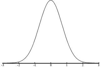
At the end of the nineteenth century, the non-fixed relationship of a sign and its ob-ject was introduced by the philosophy of language and has been widely accepted ever since. In particular, it is acknowledged that a sign is always interpreted as refer-ring to something else within a social context. For a statistician, for example, a sketch similar to Figure 1.1 signifies a normal distribution, but a student who does not know this distribution as a statistical object may interpret it as an image of a mountain. This indicates a fundamental learning problem: symbols in mathematics and statistics refer to objects that students still need to construct. This problem can supposedly be overcome if students start with simple symbols and meanings they at-tribute to them and gradually develop more sophisticated symbols and meanings. It is assumed that the process of symbolizing (making, using, and adjusting symbols) and the process of constructing meaning of such symbols co-evolve (Meira, 1995). How this co-evolvement proceeds is the theme of Chapters 8 and 9.
Figure 1.1: Graph symbolizing the normal distribution
1.4
Computer tools
Computer tools allow users to dynamically interact with large data sets and to ex-plore different representations in a way that is impossible by hand. However, com-puter tools can also distract students’ attention to the tools themselves instead of me-diating effectively between the learner and what is to be learned (Noss & Hoyles, 1996). As we establish in Section 2.2, students with hardly any statistical back-ground need special educational software to learn statistics. We are therefore inter-ested in the question of how such educational computer tools could be used to sup-port students’ learning. In the present study we used the Minitools (Cobb, Grave-meijer, Bowers, & Doorman, 1997) that were designed for the Nashville research. The Minitools are three simple applets with one type of plot for each applet, which we have translated and revised. Minitool 1 offers a value-bar graph, Minitool 2 a stacked dot plot, and Minitool 3 a scatterplot (see Section 2.3). In the present study, students only used Minitools 1 and 2.
The purpose of this research, as identified in Chapter 1, is to contribute to an empir-ically grounded instruction theory for statistics education at the middle school level. In this chapter, we begin with the pedagogical and didactical philosophy of the do-main-specific instruction theory of Realistic Mathematics Education (RME). Next we survey the research in statistics education relevant to the present study and focus on the Minitools research from Nashville that the present study builds upon. In the last section we formulate the research questions of this study.
2.1
Realistic Mathematics Education (RME)
Realistic Mathematics Education (RME) is a theory of mathematics education that offers a pedagogical and didactical philosophy on mathematical learning and teach-ing as well as on designteach-ing instructional materials for mathematics education. RME emerged from research in mathematics education in the Netherlands in the 1970s and it has since been used and extended,2 also in other countries. Some readers might wonder why we start with a theory on mathematics education as statistics is not a branch of mathematics. One reason is that contexts are very important to both the RME theory and statistics education. Moreover, educational practice is that statistics is taught as part of the mathematics curriculum.
The central principle of RME is that mathematics should always be meaningful to students. The term ‘realistic’ stresses that problem situations should be ‘experien-tially real’ for students. This does not necessarily mean that the problem situations are always encountered in daily life. Students can experience an abstract mathemat-ical problem as real when the mathematics of that problem is meaningful to them. Freudenthal’s (1991) ideal was that mathematical learning should be an enhance-ment of common sense. Students should be allowed and encouraged to invent their own strategies and ideas, and they should learn mathematics on their own authority. At the same time, this process should lead to particular end goals. This raises the question that underlies much of the RME-based research, namely that of how to sup-port this process of engaging students in meaningful mathematical and statistical problem solving, and using students’ contributions to reach certain end goals. Views similar to those within RME have been formulated in general reform efforts in the United States (NCTM, 1989, 2000), Australia (ACE, 1991), and other coun-tries, and by the theoretical movements such as situated cognition, discovery learn-ing, and constructivism in its variants. The theory of RME, however, is especially
tailored to mathematics education, because it includes specific tenets on and design heuristics for mathematics education. When we use the term ‘design’, we mean not only instructional materials, but also instructional setting, teacher behavior, interac-tion, and so on. RME tenets and heuristics are described in the following sections.
2.1.1 Five tenets of RME
On the basis of earlier projects in mathematics education, in particular the Wiskobas project, Treffers (1987) has defined five tenets for Realistic Mathematics Education:
1 Phenomenological exploration. A rich and meaningful context or phenomenon, concrete or abstract, should be explored to develop intuitive notions that can be the basis for concept formation.
2 Using models and symbols for progressive mathematization. The development from intuitive, informal, context-bound notions towards more formal mathemat-ical concepts is a gradual process of progressive mathematization. A variety of models, schemes, diagrams, and symbols can support this process, provided these instruments are meaningful for the students and have the potential for gen-eralization and abstraction.
3 Using students’ own constructions and productions. It is assumed that what stu-dents make on their own is meaningful for them. Hence, using stustu-dents’ con-structions and productions is promoted as an essential part of instruction. 4 Interactivity. Students’ own contributions can then be used to compare and
re-flect on the merits of the different models or symbols. Students can learn from each other in small groups or in whole-class discussions.
5 Intertwinement. It is important to consider an instructional sequence in its rela-tion to other domains. When doing statistics, what is the algebraic or scientific knowledge that students need? And within one domain, if we aim at understand-ing of distribution, which other statistical concepts are intertwined with it? Math-ematics education should lead to useful integrated knowledge. This means, for instance, that theory and applications are not taught separately, but that theory is developed from solving problems.
In addition to these tenets, RME also offers heuristics or principles for design in mathematics education: guided reinvention, didactical phenomenology, and emer-gent models (Gravemeijer, 1994). We describe these in the following sections.
2.1.2 Guided reinvention
invented (Gravemeijer, 1994). The designer of realistic mathematics instruction can use different methods to design instruction that supports guided reinvention. The first method is what Freudenthal called a ‘thought experiment’: designers should think of how they could have reinvented the mathematics at issue themselves. In fact, this is what Freudenthal (1991) used to do when he read mathematical theo-rems: find his own proof of the theorems. The second method is to study the history of the topic at issue: the method of carrying out a so-called historical phenomenolo-gy is used in Chapter 4. The third method, elaborated by Streefland (1991), is to use students’ informal solution strategies as a source: how could teachers and designers support students’ solutions in getting closer to the end goal?
2.1.3 Didactical phenomenology
To clarify his notion of phenomenology, Freudenthal (1983a) distinguished thought objects (nooumena) and phenomena (phainomena). Mathematical concepts and tools serve to organize phenomena, both from daily life and from mathematics itself. A phenomenology of a mathematical concept is an analysis of that concept in rela-tion to the phenomena it organizes. This can be done in different ways, for example:
1 Mathematical phenomenology: the study of a mathematical concept in relation to the phenomena it organizes from a mathematical point of view. The arithmet-ical mean is used, for example, to reduce errors in astronomarithmet-ical observations. See Section 5.2 for a short mathematical phenomenology of distribution.
2 Historical phenomenology: the study of the historical development of a concept in relation to the phenomena that led to the genesis of that concept. For example, the mean evolved from many different contexts, including navigation, metallur-gy, and astronomy. It took until the sixteenth century before the mean of two val-ues was generalized to more than two valval-ues. The first implicit use was in esti-mating large numbers (Section 4.3.1).
3 Didactical phenomenology: the study of concepts in relation to phenomena with a didactical interest. The challenge is to find phenomena that “beg to be organ-ised” by the concepts that are to be taught (Freudenthal, 1983a, p. 32). In Section 6.2 we describe how students organized a picture of elephants into a grid and used a so-called ‘average box’ to estimate the total number of elephants in the picture.
be generalized to other problem situations. This last possibility is worked out under the heading of emergent models.
2.1.4 Emergent models
As the second tenet of RME about models for progressive mathematization implies, we search for models that can help students make progress from informal to more formal mathematical activity. Gravemeijer (1994, 1999a) describes how models of
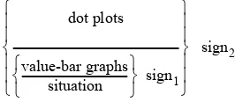
a certain situation can become a model for more formal reasoning. In the case of sta-tistics, the notion of a distribution in combination with diagrams that display distri-butions was envisioned to become a model of data sets and later a model for more formal statistical reasoning (Gravemeijer, 2002).
Figure 2.1: Levels of emergent modeling from situational to formal reasoning.
These four levels (Figure 2.1) can be described as follows (after Gravemeijer, Cobb, Bowers, & Whitenack, 2000, p. 243):
1 Situational level: activity in the task setting, in which interpretations and solutions depend on understanding of how to act in the setting (often in out-of-school set-tings);
2. Referential level: referential activity, in which models-of refer to activity in the setting described in instructional activities (mostly posed in school);
3. General level: general activity, in which models-for enable a focus on interpreta-tions and soluinterpreta-tions independently of situation-specific imagery;
4. Formal level: reasoning with conventional symbolizations, which is no longer de-pendent on the support of models-for mathematical activity.
2.2
Trends in statistics education research
Now that we have discussed the domain-specific theory of RME, we move to the do-main of statistics education. This section gives an overview of research in statistics education relevant for the present study. Concentrating on research at the middle school level, when students are about 10 to 14 years old, we do not pay much atten-tion to issues such as assessment (Gal & Garfield, 1997) and professional develop-ment of teachers (Mickelson & Heaton, in press; Makar & Confrey, in press), al-though these are important topics of research.
1. situational 2. referential 3. general
As background information we first sketch a short history of statistics education in the Netherlands. Statistics was proposed as part of the secondary mathematics cur-riculum in 1954, but the proposal was rejected due to concerns about an overloaded curriculum. It was not until the early 1970s that descriptive statistics was introduced in the upper-levels of the secondary mathematics curriculum. The main reasons for introducing statistics in the curriculum were that it was needed in many sciences and fields of work and that students could experience the usefulness of mathematics (Freudenthal, 1974; Van Hiele, 1974). Around 1990, statistics was introduced in the lower grades; since then graphs such as the box plot and the stem-and-leaf plot have been taught in grade 9 (W12-16, 1992).
We start our overview of research in statistics education with the work of Kahne-man, Tversky, and their colleagues because much of the early research in statistics education was grounded in their work (Kahneman & Tversky, 1973, 1982; Shafir, Simonson, & Tversky, 1993; Tversky & Kahneman, 1971, 1982; Tversky & Shafir, 1992). From the early 1970s onwards, these cognitive psychologists have been in-vestigating how people use statistical reasoning in everyday situations to arrive at decisions. Although these heuristics result in the same decisions as would be made based on statistical theory, there are instances when they lead to decisions which are at odds with such theory.3 The overall impression is that statistical reasoning is very demanding cognitively.
In the late 1970s and 1980s, statistics education research mainly focused on college level and on probability (Pfannkuch & Wild, in press). In the 1990s, studies were un-dertaken at lower levels, mainly middle school level, and because statistics became part of the mathematics curriculum, more and more mathematics educators became involved in the discipline. Because statistics appeared early in the curriculum of the United States, Australia, and the United Kingdom, the majority of studies at the mid-dle school level took place in these countries.
When we compare the curricula of different countries, for instance, the United States, the Netherlands, and Germany, we can observe a lot of variation. In the Unit-ed States, mean, mUnit-edian, and mode are introducUnit-ed in grade 4 or 5, when students are 9 or 10 years old (NCTM, 2000). In the Netherlands, students learn their first de-scriptive statistics in grade 8, when they are 13 or 14 years old. In most German states, the median is not even in the high school curriculum (Engel, personal com-munication, November 4, 2002).
These international differences in curricula indicate that we cannot simply apply re-search findings from, for instance, American studies to the Dutch situation. If Dutch students learn a statistics topic in a higher grade than American students, the Dutch students will mostly have a better mathematical background than American students in lower grades, which could make it easier (or perhaps more difficult) to learn
tain statistical topics. Mathematical issues that have been identified as important for statistics are multiplicative reasoning (ratios, percentages, and proportions), the Car-tesian system, and line graphs (Cobb, 1999; Friel, Curcio, & Bright, 2001; Zawojew-ski & Shaughnessy, 1999). On the one hand, this means that Dutch students with proficiency in these matters do not necessarily encounter the same problems with statistical graphs and concepts as younger American students. On the other hand, the Dutch seventh-grade students do not have the same experience with data and science as most younger American students. This reveals the need for design research that will eventually lead to statistics curricula that are tuned to the mathematics and sci-ence curricula in the different countries.
The prominent image that emerges from reading the early research on statistics ed-ucation is that students have trouble with understanding and using the mean, which was the most investigated statistic. Students mostly know how to calculate it but are not able to use it well (Hardiman, Well, & Pollatsek, 1984; Mevarech, 1983; Mokros & Russell, 1995; Pollatsek, Lima, & Well, 1981; Strauss & Bichler, 1988). Similar problems occur for many statistical graphs such as the histogram and for methods such as hypothesis testing. The literature gives the impression that students had to deal with artificial problems and artificial data (Singer & Willett, 1990), that statis-tics consisted of ‘number crunching’ (Shaughnessy, Garfield, & Greer, 1996, p. 209) and that statistics courses were overloaded with formal probability theory, which led to the nickname of ‘sadistics’ (Wilensky, 1997). With these images in mind, we summarize recent developments in statistics education research with the following five trends.
1 New pedagogy and new content; 2 Using exploratory data analysis (EDA); 3 Using technology;
4 Focusing on graphical representations;
5 Focusing on aggregate features and key concepts.
1. New pedagogy and new content. In the research literature, the information trans-mission model has made place for constructivist views, according to which students should be active learners (Moore, 1997). Bottom-up learning is advocated as op-posed to top-down teaching. Students should have the opportunity to explore, build upon their intuitive knowledge, and learn in authentic situations. Such ideals are also expressed in the reform movements in mathematics education (NCTM, 2000) and the theory of Realistic Mathematics Education (2.1).
advo-cates a similar view for statistics education: statistics is often taught as a set of tech-niques, but these ‘one-shot’ standard ways of dealing with certain situations such as hypothesis testing are often black boxes to students, and do no justice to the practice of statistical investigations either. An example of the new pedagogy and content is given by De Lange and colleagues (1993), who report that students can reinvent meaningful graphs themselves.
A call for new pedagogy and content also came from a different source. Although statistics was (and still is) often taught as if it were a branch of mathematics, many statisticians have argued that it should be taught differently. G. Cobb (1997), for ex-ample, has spelled out the implications of this view for statistics education: where mathematics focuses on abstraction, statistics cannot do without context. One of his slogans to summarize this view was “more data and concepts, less theory and reci-pes” (see also G. Cobb & Moore, 1997). The emergence of constructivist philosophy and exploratory data analysis fitted well with these attempts to differentiate statistics from mathematics.
2. Exploratory data analysis (EDA) is a relatively new area of statistics, in which data are explored with graphing techniques (Tukey, 1977). The focus is on meaning-ful investigation of data sets with multiple representations and little probability the-ory or inferential statistics. In EDA, it is allowed to look for unanticipated patterns and trends in existing data sets, whereas traditional inferential statistics only allows testing of hypotheses that are formulated in advance.
EDA was adopted by several statistics educators to serve the need for more data and less theory and recipes (Biehler, 1982; Biehler & Steinbring, 1991). EDA was also thought useful to bridge the traditional gap between descriptive and inferential sta-tistics. Descriptive statistics was often taught as too narrow a set of loosely related techniques, and inferential statistics tended to be overloaded with probability theory. EDA was considered an opportunity to actively involve students, to broaden the con-tent of descriptive statistics, to give students a richer and more authentic experience in meaningful contexts, and to come closer to what statistics is really about (Ben-Zvi & Arcavi, 2001; Jones et al., 2001; Shaughnessy et al., 1996). Manually exploring real data with graphing techniques is laborious, which implies that using technology is a big advantage.
of knowledge and they should have the opportunity to experience mathematics as meaningful, but computer software mostly seems to provide the opposite: what is possible in a software program is predetermined, and what the computer does in re-action to clicking certain buttons can hide the conceptually important part of the op-erations (cf. Drijvers, 2003, about computer algebra systems). Of course, students need not know exactly which operations the software does to make a histogram, but they should be able to understand that data are categorized into certain intervals and that the bars’ areas are relative to the number of values in those classes. In most sta-tistical software packages such operations are hidden, which suggests that we need special software for education that minimizes this black-box character. As Biehler writes:
Professional statistical systems are very complex and call for high cognitive entry cost. They are often not adequate for novices who need a tool that is designed from their bottom-up perspective of statistical novices and can develop in various ways into a full professional tool (not vice versa). (…) As a rule, current student versions of pro-fessional systems are no solution to this problem because they are technical reductions of the complete system. (Biehler, 1997, p. 169)
In Sections 2.3, we discuss bottom-up software tools that have been designed spe-cially for middle school students and that have been used in this study, the Minitools (another bottom-up program, Tinkerplots (Konold & Miller, 2004), is under devel-opment). The present research focuses on cognitive tools (Lajoie & Derry, 1993), not on simulations, computer-based instruction, or web-based projects. We are in-terested in how educational tools can be used in a sensible way and ask what the graphs provided by these tools mean to students. These computer programs and graphs are tools that reorganize learning. We deliberately avoid ‘amplify’ or ‘im-prove learning’, because numerous researchers have shown that using computer tools often drastically changes the learning process and what is learned (e.g. Dörfler, 1993; Noss & Hoyles, 1996; Pea, 1987). It can be hard to compare statistical learning with and without the use of technology, because these two conditions lead to the learning of different ‘content’, which is, as noted above, often inseparable from the tools and symbols used (cf. Tall et al., 2000). In the present research, we ask how
computer tools can be used, not whether using computer tools leads to better test re-sults.
is not a feature of the graph itself, but that it is connected to a purpose and tied to a cultural practice. Meira (1998) describes transparency as an emergent phenomenon intricately interwoven with learners’ current activities and participation in ongoing cultural practices (see also Roth, 2003). This means that a graph is not an end goal in itself but that it should serve the purpose of solving a statistical problem and com-municating the results. Even then, as Lehrer and Schauble (2001) note, graphs are too often taught as prefabricated solutions that have advantages and conventions that may be invisible to students. The question that rises is how can we let students rein-vent and use graphical tools for statistical problem solving and in which order can we provide them with graphical tools that are meaningful for them.
Several researchers have proposed a certain order of graphs based on the complexity of the graphs for students (Biehler & Steinbring, 1991; Friel, Curcio, & Bright, 2001). Feldman, Konold, and Coulter (2000) suggest an order that is based on how easy it is to identify individual cases in a plot. Cobb, McClain, and Gravemeijer (2003) proposed a sequence of graphs, value-bar graphs before dot plots, which is summarized in the next section.
A conclusion we have drawn from several studies is that students should begin with graphs in which they can retrace each individual data value, so-called ‘case-value plots’, before they use graphs in which data are aggregated, so-called ‘aggregate plots’ (Konold & Higgins, 2003). Typical examples of case-value plots are case-val-ue bar graphs (Figure 2.2) and stacked dot plots (Figure 2.3); examples of aggregate plots are histograms and box plots. Bar graphs can be both case-value plots and ag-gregate plots. If each bar represents a case, it is a case-value plot (a case-value bar graph, as Feldman et al., 2000, call it). If a bar represents a number of cases, a fre-quency for instance, it is an aggregate plot. A consequence of this is that using graphs such as histograms and box plots is more demanding for students than using bar graphs and dot plots. But there is more. There are hidden conventions and con-ceptual elements in histograms and box plots: in histograms, the area of the bars is relative to the number of values it signifies, and in box plots conceptual elements such as median and quartiles are depicted.
The difference in case-value and aggregate plots highlights that students need con-ceptual structures to conceive aggregates before they can interpret and use graphs sensibly. This insight explains the focus on aggregates and the key concepts of sta-tistics at the middle school level (trend 5). In fact, this is the reason that we have a closer look at the relationship of graphs and concepts in the process of symbolizing and ask how we can support students in developing an aggregate view on data. 5. Focus on aggregate features and key concepts. Statistical data analysis is mainly about describing and predicting aggregate features of data sets.
One can mostly not predict the values of individual cases, but one can predict aggre-gate features such as the mean or the distribution of a data set. Hancock, Kaput, and Goldsmith (1992) note that students have considerable trouble in conceiving data sets as aggregates. This implies that there is a strong conceptual component in inter-preting graphs: in order to be able to see the aggregate students have to ‘construct’ it. After Hancock and colleagues, other researchers have dealt with the problem as well. Konold, Pollatsek, and Well (1997), for example, observed that high school students, after a yearlong statistics course, still had a tendency to focus on properties of individual cases, rather than on propensities of data sets. Ben-Zvi and Arcavi (2001) notice that seventh-grade students initially have a local view on data, and need time and good support to develop a global view on data. Without appropriate conceptual structures, students do not perceive the data as is necessary for doing sta-tistical data analysis.
This stresses the necessity of addressing a number of key concepts of statistics, which are also called ‘overarching statistical ideas’ or, with a somewhat fashionable term, ‘big ideas’ (Schifter & Fosnot, 1993). There is no unique list of the key con-cepts of statistics. Here, we advocate a list for the middle school level that is inspired by a list from Garfield and Ben-Zvi (in press) for statistics education in general. We do not want to suggest any order, because these key concepts are only meaningful if dealt with in relation to each other (Wilensky, 1997).
– Variability; – Sampling; – Data; – Distribution; – Covariation.
Variability
Variability is at the heart of statistics because without variability there is no need for statistical investigation (Moore, 1990). In the PISA framework for assessment in mathematics education (OECD, 1999), statistics and probability fall under the over-arching idea of ‘uncertainty’ (the others being ‘change and growth’, ‘shape and space’, and ‘quantitative reasoning’). Kendall characterized statistics as the science that gives relative certainty about uncertainty.
We live in a world of chance and change, surrounded by uncertainty; our object is to impose a purpose on that uncertainty and, in some sense, to bring the world under con-trol (Kendall, 1968, p.1)
vari-ability. If we plan to go somewhere by car, for example, it is uncertain at what time we will arrive due to variability among conditions. Various uncertain factors, such as traffic jams and weather conditions cause variability in travel times. We chose to call this key concept ‘variability’ because ‘uncertainty’ has the connotation of prob-ability, which we do not address in this thesis.
Sampling
In order to investigate a variable phenomenon, one can take a sample. Without pling there is no data set, distribution, or covariation to describe. The notion of sam-pling has been studied at the middle school level, but not extensively. Though stu-dents seem to have useful intuitions about sampling, it is a complex notion that is difficult to learn (Rubin, Bruce, & Tenney, 1990; Schwartz et al., 1998; Jacobs, 1999; Watson & Moritz, 2000; Watson, 2002).
Data
Sampling and measurement lead to data, that is numbers with a context (Moore, 1997). The idea of data involves insight into why data are needed and how they are created. This implies that the idea of data relies on knowledge about measurement. Too often, however, data are detached from the process of creating them (Wilensky, 1997), so many researchers and teachers advocate students collecting their own data (NCTM, 2000; Shaughnessy et al., 1996). This is time-consuming, so “talking through the process of data creation,” as Cobb (1999) calls it as opposed to data col-lection, can sometimes substitute for the real creation of data. Once represented as icons, we can manipulate the data icons in a graph to find relations and characteris-tics that are not visible from the table of numbers (Lehrer & Romberg, 1996). The idea of data is intimately connected with the other overarching ideas. For in-stance, data are often conceptually organized as ‘pattern + deviation’ (Moore, 1997) or as ‘fit + residual’ (G. Cobb, 1997) and data analysis is also described as the search for signals in noisy processes (Konold & Pollatsek, 2002). A data set can be ana-lyzed for patterns and trends by using suitable diagrams. A key instrument in this analysis process is the concept of distribution with its various aspects such as center and spread.
Distribution
Distribu-tion could afford an organizing conceptual structure for thinking about patterns in variability and to view a data set as an aggregate. Besides that, distribution is a key idea in statistics that is connected to almost all other statistical concepts. Hence, fo-cusing on distribution as an end goal of instruction or as a guideline for design has the additional advantage of possibly providing more coherence in the different sta-tistical concepts and graphs (Cobb, 1999).
Because distribution is a complex concept with many aspects and different layers of possible understanding, from frequency distributions to probability density func-tions, research is needed to tease out the different conceptions of distribution that students have and can develop. The historical study in Chapter 4 aids in the analysis of this concept. Section 5.2 is devoted to this key concept of distribution, in partic-ular the necessity of viewing a data set as a whole or an object that can have charac-teristics. A central question of the present study is how this process of becoming an object (reification) evolves (Chapter 8 and 9).
We consider center and spread as two main characteristics of the concept of distri-bution.
Center
Center can only be the center of something else, the distribution. If there is a ‘true value’, a measure of center can be used to estimate the signal in the noise (Konold & Pollatsek, 2002). However, as Zawojewski and Shaughnessy (2000) argue, stu-dents can only sensibly choose between the different measures of center if they have a notion of the distribution of the data.
Spread
Spread did not receive much attention in statistics education research until about 1997 (Shaughnessy, Watson, Moritz, & Reading, 1999; Reading & Shaughnessy, 2000). The reason for neglecting spread in education has probably been the focus on the measures of central tendency. We use the term spread for variation in the variable at issue, and ‘variation’ as a more general term, for example for variation in frequen-cy, in density, or around a curve. Noss, Pozzi, and Hoyles (1999) report on nurses who view spread as crucial information when investigating blood pressure. Spread is also crucial information when doing repeated measurements, for example in a physical or biological context (Lehrer & Schauble, 2001). For an overview of the re-search on variation see Meletiou (2002).
Statisticalcovariation
idea. They are convinced that students should first develop a notion of univariate dis-tributions before they can sensibly deal with covariation. It is perhaps not too diffi-cult to draw a straight line by eyeballing, but Cobb and colleagues chose to deal with covariation at a deeper level than just drawing a line through a cloud to signify a trend.
Covariation is not a topic investigated in the present study. We focused on the first four key concepts, because the students hardly had any statistical background and had only 10 to 15 lessons on data analysis (it was not possible to use more lessons). We do mention covariation as a key concept, because we think that it should be somewhere in the Dutch mathematics curriculum: students encounter covariation in physics, chemistry, biology, and the social sciences, mostly represented in scatter-plots.
There is not much research on how these key concepts can be developed at the mid-dle school level. If we narrow our focus to studies that use bottom-up software in which students do not have to choose from ready-made graphs, the only one research we can directly build upon is that of the research team in Nashville (e.g. Cobb, Mc-Clain, & Gravemeijer, 2003). That research focused on the notion of distribution (grade 7) and covariation (grade 8), and, as mentioned in Chapter 1, formed the start-ing point of the present study.
In the next section, we summarize the results of the Nashville research in a very de-tailed way, which allows us to present elements of our initial conjectured instruction theory for early statistics education and to confirm, reject, or extend their findings.
2.3
Nashville research with the Minitools
In this section,4 we summarize the instructional design issues of the research carried out by Cobb, McClain, and Gravemeijer and their team at Vanderbilt University, Nashville, USA. We focus on their points of departure (2.3.1), the rationale of the software (2.3.2), results and recommendations (2.3.3), and the way they described the process of symbolizing (2.3.4). The numerous articles on these teaching experi-ments mainly deal with themes that transcend the instructional design issues that we are interested in here: individual and collective development of mathematical learn-ing, sociomathematical norms and mathematical practices, tool use, the teacher’s proactive role, diversity, equity, and so on. We therefore base this section mainly on Gravemeijer’s manuscripts on the instructional design part of the research (Grave-meijer, 1999b, c, 2000a, b, 2001) and thus make the instructional design component accessible to a wider audience. Other sources used for this section were videotapes of the seventh-grade teaching experiment and articles that have been published (Cobb, 1999, 2002; Cobb & Hodge, 2002a, 2002b; Cobb & McClain, 2002, in press;
Cobb, McClain, & Gravemeijer, 2003; Cobb & Tzou, 2000; Gravemeijer, 2001, 2002; McGatha, 1999; McClain, 2002; McClain & Cobb, 2001; McClain, McGatha, & Hodge, 2000; McGatha, Cobb, & McClain, 2002; Sfard, 2000a). We start with factual information about the teaching experiments with the Minitools.
Members of the research team at the Vanderbilt University, Nashville, TN, USA, were Paul Cobb, Kay McClain, Koeno Gravemeijer, Maggie McGatha, José Corti-na, Lynn Hodge, Carrie Tzou, Carla Richards, and Nora Shuart-Farris. External con-sultants were Cliff Konold (University of Massachusetts, Amherst) and Erna Yackel (Purdue University, Calumet). A short pilot with seventh-graders (twelve years old) was carried out in the fall of 1996 (McGatha et al., 2002). The seventh-grade teach-ing experiment took place in a regular school situation in the fall of 1997 and con-sisted of 37 lessons of 40 minutes, with a group of 29 students over a ten-week pe-riod; the eighth-grade teaching experiment was one year later in 1998 with 11 of the 29 students (thirteen years old) and consisted of 41 lessons of 40 minutes over a four-teen-week period. This last experiment was carried out during the so-called ‘activity hour’, normally used for doing homework. The school served a mixed working class and middle class student population, and about 40% of the students were classified as minority (almost all African American). In the course of the experiment, 5 stu-dents dropped out and 11 voluntarily continued to attend throughout (Cobb, personal communication, November 22, 2002).
2.3.1 Points of departure and end goal
con-cepts when they learn to analyze data (trend 5). Otherwise, they would probably keep perceiving individual data instead of conceiving the aggregates displayed in the graphs.
We have numbered the issues to refer more easily to the same issues later in this book when we show how our results compare to those of the Nashville team. P# stands for point of departure number #, and R# for result or recommendation number #. We would like to draw attention to the fact that the first teaching experi-ment took place in 1997, when much less was known about statistics education than nowadays, and that issues in this section should be seen as part of a design process.
P1. As pointed out, EDA requires conceptual tools to conceive of patterns and trends. The research team decided to combine, as they called it, the process charac-ter of EDA with the product character of statistical tools and concepts as endpoints of instruction (Gravemeijer, 2000a; McGatha et al., 2002).
P2. The pedagogical point of departure was that the learning process should always be genuine data analysis from the outset, as opposed to learning specific tools and then applying them. Students should deal with real problems that they considered so-cially important or, in other words, a statistical problem had to be solved for a rea-son. This point of departure influenced the contexts that were used (AIDS, ambu-lance travel times, CO2 emission, speeding cars, braking distances of cars).
P4.Instructional format. The instructional format typically used was a whole-class discussion, followed by individual or group work with computers, and again a whole-class discussion. The first discussion was for talking through the data creation process and the second discussion was for collectively discussing students’ analyses.
P5.Distribution. With these points of departure, the question was, “Which concepts and graphical tools do we have to focus on?” In her dissertation on the learning of the research team, McGatha (1999) describes how the notion of distribution as a po-tential end goal of the instructional sequence emerged from a conceptual analysis of the topics and from the discussion on the relevant research literature. The two major reasons to focus on distribution were the following.
First, distribution is a concept that can help students to conceive aggregates. Data had to be seen as distributed in a space of possible values and the notion of distribu-tion had to become, in the end, an object-like entity with characteristics such as where the data were centered and how they were spread. Conventional graphs such as box plots and histograms had to emerge as ways to describe and structure distri-butions. A more extensive analysis of this notion of distribution is given in Section 5.2.
Second, focusing on distribution could bring more coherence to the curriculum. Tra-ditionally, statistical concepts and graphs are taught in middle school as a set of loosely related techniques (Cobb, 1999). Concepts such as mean, median, spread, and skewness are only meaningful when they refer to distributions. Coherent statis-tical knowledge could emerge if these concepts can be developed as characteristics of distributions and graphs as ways to structure and describe distributions.
P6. The team conjectured that comparing distributions would be a valuable way to involve students in reasoning about characteristics of distribution, because there would be a reason to think about the whole data sets.5 Hence, most instructional ac-tivities in the seventh-grade experiment involved comparing two distributions.
P7.Mean. There were three reasons not to focus on the mean. The first reason was that a considerable amount of research, including an analysis of the pilot (McGatha et al., 2002), showed that students generally see the mean as a procedure and do not use it sensibly to compare groups (see also Section 2.2). The team thought that this procedural approach would interfere with the kind of reasoning they wanted to fos-ter. Gravemeijer (1999b):
Another reason for avoiding the mean was in our assertion that the mean is not very relevant if it comes to characterizing the distribution of data values. The mean does
give you an aggregated measure of the data values but it does not tell you anything about the distribution as such. (p. 13)
As we explain in Chapters 4 and 5, this is not our own view.
P8. The median seemed more appropriate to use as a measure of center than the mean, and quartiles seemed more appropriate to use as a measure of spread than the standard deviation (Gravemeijer, 1999b). In the team’s reasoning, the median was easier to understand than the mean (but see R16), the position of the median in rela-tion to the extreme values showed skewness, and a five-number summary of mini-mum, first quartile, median, third quartile, and maximum was seen as a way to de-scribe the distribution (Tukey, 1977).
P9.Sampling. EDA typically does not deal with probability and sampling issues. G. Cobb and Moore (1997), writing about college level, recommend EDA as a basis for data production (design), which in turn forms the basis for probability and then sta-tistical inference. Because the research team brought distribution and multiplicative reasoning to the foreground, the issue of sampling moved to the background and was not to be addressed explicitly.
P10. The designers experienced that it was almost impossible to find real data sets that served their pedagogical agenda. This was the reason they mainly used realistic
data as opposed to real data, where realistic means “as it could have been in a real situation.”
P11. Multiplicative reasoning. During the pilot, the team had noticed that students struggled with ratios and proportions when solving statistical problems. Students’ reasoning is called additive if they use absolute instead of relative frequencies. For instance, if students compare 4 of a group of 24 with 6 of a group of 65 without tak-ing the proportion into account, they reason additively. If they use proportions or percentages to compare the groups of different size, they reason multiplicatively (cf. Thompson, 1994). Konold et al. (1997) argue that a focus on a proportion of data within a range of values is at the heart of a statistical perspective, so multiplicative reasoning is an important issue to address. Multiplicative reasoning “also cuts across a number of content strands and constitutes the overarching goal for American math-ematics instruction at the middle-school level” (McClain & Cobb, 2001, p. 108). The team therefore decided to make multiplicative reasoning a central theme of the re-search.
The problem of technology as described in trend 3 implied that special software had to be designed. This is the topic of the next section, which also deals with the repre-sentational backbone of the instructional sequence. The specially designed so-called ‘Statistical Minitools’ (Cobb, Gravemeijer, Bowers, & Doorman, 1997) were used in 27 of the 34 classroom sessions of the seventh-grade experiment, and in about 25 of the 41 sessions of the eighth-grade experiment.
2.3.2 Rationale of the Statistical Minitools6
Most educational statistical software packages only provide common and culturally accepted graphical representations (e.g. Datascope, Fathom, VU-Stat; see also Bie-hler, 1997). Users of such packages need to anticipate the information that they can extract from the representations and measures that the computer program has to of-fer. For students with hardly any statistical background, this is difficult, and such an approach is not in line with the reform movements or the RME philosophy. Tabletop (Hancock, 1995) does offer non-standard plots, but in the team’s view this program seemed to orient students to focus on characteristics of individual cases, which was at odds with their concern for distribution. The team therefore developed three so-called Statistical Minitools to support a process of guided reinvention of the notion of distribution and graphical representations that can organize distributions. The backbone of the sequence is formed by a series of inscriptions that are embedded in the Minitools.
Figure 2.2: Case-value bars in Minitool 1 signifying life spans in hours of two different battery brands
The rationale is that the activities with the computer tools follow each other in such a manner that the activity with the newer tool is experienced as a natural extension of the activity with the earlier tool.
Minitool 1
The starting point is in the measures, or magnitudes, that constitute the data set. With Minitool 1, case-value bars (Figure 2.2) are introduced that signify single measures. Initially, the measures under investigation are of a linear type, such as length and time. Later, this is generalized to other types of measures. Students can organize the data by sorting by size and by color (for comparing subsets). Furthermore, there are two tools, a ‘value tool’ and a ‘range tool’, which have to support the organization of data and understanding of the variable on the horizontal axis. The value tool (or ‘reference line’) was also meant to afford visual estimation of a measure of center, in particular to avoid calculations for getting the mean. The range tool was to support the discourse on a modal class.
Figure 2.3: A dot plot in Minitool 2
Minitool 2
dot plot. Note that there is no frequency axis: the students still need to construct one mentally. This type of representation is also called a numberline plot.7
Minitool 2 offers various tool options to help the students structure the distribution of data points in a dot plot. There are five options to structure the data: making your own groups, making two or four groups with an equal number of data points, making groups of a certain size (e.g. 10 data points per group), and making equal intervals.
Create your own groups. Apart from incorporating options that would anticipate conventional graphs, the team wanted to make sure that the Minitool would offer the students the freedom to structure the data in ways that make sense to them. Hancock and colleagues had observed that students tend to make their own clusters of data (Hancock, Kaput, & Goldsmith, 1992), so an option to create one’s own groups was built in.
Two and four equal groups. Minitool 2 features equal-groups options, one that par-titions a set of data points into two halves, and one that parpar-titions a set of data points into four quartiles. The latter results in a four-equal-groups inscription, which can be seen as a precursor to the conventional box plot. The similarity with a box plot is clearer when the ‘hide data’ option is used (Figure 2.4).
Figure 2.4: Dot plot structured into four equal groups and with ‘hide data’
Figure 2.5: Box plot overlay that was made available in the revised version of Minitool 2
The hide data option also creates the opportunity to shuttle back and forth between the dot plot and the four-equal-groups inscription. This is helpful, for instance, if one wants to make the adequacy of a four-equal-groups description a topic for discus-sion. The four-equal-groups option was considered useful for fostering multiplica-tive reasoning: it does not depend on the size of the data set, so data sets of different size can be compared adequately. The team assumed that the four-equal-groups in-scription (a precursor to the box plot) would support reasoning about the shape of the distribution in terms of density, which is a key characteristic of a distribution. The idea is that students learn to relate the width of an interval to the density of the distribution in that area.
Equal interval width. As an alternative to the four-equal-groups option, the students can also choose to structure the data in equal intervals. When using this option, the students can indicate the size of the interval width. In addition to intervals, Minitool 2 shows the number of data points in each interval (Figure 2.6).
Figure 2.6: Dot plot structured into equal intervals and with ‘hide data’
Figure 2.7: The histogram overlay that was made available in the revised version of Minitool 2
see the shape of the dot plot as a description of the distribution of variable values in terms of density” (Gravemeijer, 2000b). The box plot and the histogram overlays (Figures 2.5 and 2.7) were not available in the original version of Minitool 2; they were added during the present research, but only the eighth graders worked with them.
Minitool 3
For the eighth-grade experiment in Nashville, the end goal was that students would come to see bivariate data as a series of distributions of univariate data. To support a learning process towards that end goal, Minitool 3 was developed. It offered a scat-terplot with a few ways of structuring the data such as groups of a fixed size or equal groups. One insight was that a series of stacked distributions (as in Figure 2.8) would support deeper understanding of covariation in a scatterplot (Cobb, McClain, & Gravemeijer, 2003). Deeper understanding meant that covariation had to be much more than drawing a line through a cloud of dots. In the team’s view, covariation in a scatterplot can be seen as a description of how a univariate distribution changes along with the independent variable. This underlines the importance of a good un-derstanding of univariate distributions before addressing statistical covariation. For this transition students need to see a series of dot plots turned at angles and squeezed into one vertical line.
Because Minitool 3 was not used in the present study, we do not discuss this Mini-tool any further (see for instance www.wisweb.nl). We only discuss the findings when students worked with Minitool 3 that were relevant for our own study.
Figure 2.8: Scatterplot in Minitool 3 with stacked data as opposed to a ‘clouds’ (left) and four equal groups within the scatterplot slices (right)
2.3.3 Results and recommendations
Seventh-grade teaching experiment
R1. Cobb and Tzou (2000) claim that talking through the data creation process
proved successful. One sign of that is that students adopted the teacher’s questioning attitude on the data creation.
R2. It was noted in retrospect that talking through the data creation process is a way of implicitly addressing the issue of sampling. However, it was acknowledged that sampling should be addressed more thoroughly, since it underlies the notion of fair comparison and it cannot always be kept in the background (Gravemeijer, 1999c). This issue is revisited in R17.
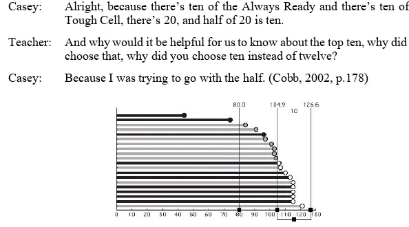
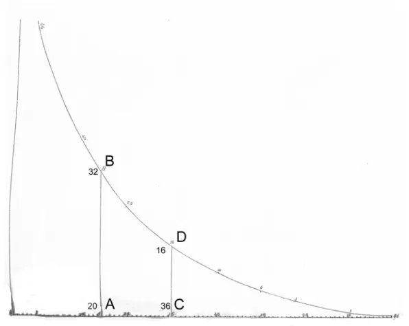
R3. The students used the range tool to partion data sets and to isolate intervals to make comparisons as well as to investigate consistency. For example, in the context of the life span of two battery brands (Always Ready and Tough Cell), Casey used it to indicate the interval 104.9 to 126.6 (Figure 2.9):
Casey: Alright, because there’s ten of the Always Ready and there’s ten of the Tough Cell, there’s 20, and half of 20 is ten.
Teacher: And why would it be helpful for us to know about the top ten, why did you choose that, why did you choose ten instead of twelve?
Casey: Because I was trying to go with the half. (Cobb, 2002, p.178)
Figure 2.9: Battery data set in Minitool 1 with range tool
R4. The value tool or vertical reference line was used to find certain values or to rea-son with certain cutting points. For example, Brad used it at 80 (Figure 2.9):
Brad: See, there’s still green ones [Always Ready] behind 80, but all of the Tough Cell is above 80. I would rather have a consistent battery that I know will get me over 80 hours than one that you just try to guess.
Teacher: Why were you picking 80?
Brad: Because most of the Tough Cell batteries are all over 80. (Cobb, 2002, p. 178)
a whole. “The mathematical practice that emerged as the students used the first mini-tool can (...) be described as that of exploring qualitative characteristics of collec-tions of data points” (Cobb, 2002, p. 179). The term ‘collection of data points’ is used here in opposition to ‘distribution’. The first term refers to additive reasoning whereas the second denotes multiplicative reasoning. The notion of the majority of data did not become a topic of discussion until students analyzed data sets with un-equal numbers (Cobb, 2002) and the notion of majority was then used in conjunction with the hill notion (see next item).
R6. In the context of comparing situations before and after the installment of a speed trap, one student spontaneously used the notion of a ‘hill’ to refer to the majority of the data points. The meaning attributed to the hill, was more than just visual; it was interpreted in the context of the speed of cars (Figure 2.10):
Janice: If you look at the graphs and look at them like hills, then for the before group the speeds are spread out and more than 55, and if you look at the after graph, then more people are bunched up close to the speed limit which means that the majority of the people slowed down close to the speed limit. (Cobb, 2002, p. 180)
In describing hills, Janice had reasoned about qualitative relative frequencies. This notion of the majority of the data, however, did not become a topic of discussion un-til the students analyzed data sets with unequal numbers of data values.
Figure 2.10: Speed trap data set in Minitool 2 (in miles per hour).
dis-tributions (Cobb, 2002). Note that this second mathematical practice is about distri-butions, whereas the first practice is about collections of data points.
R7.Bottom-up approach. The team has been reasonably successful in the bottom-up approach. The first example that supports this claim is that students themselves came up with the notion of consistency to denote what we would perhaps call the variation or spread of the data. The second example is students’ spontaneous use of the notion of a ‘hill’ for comparing distributions (see student quotes in R6).
R8.Multiplicative reasoning versus distribution. Gravemeijer (2000b) remarks that when students use Minitool 2 grouping options, there is a pitfall of fragmentation, because students often compared vertical slices. For instance, students noticed that 50% of one data set was below a certain cutting point whereas 75% of the other data set was below the same point. Hence, the development of multiplicative and arith-metical reasoning had some success at the expense of developing the notion of dis-tribution as a whole in relation to shape. See also R13.
R9. Students did not use the value tool to estimate means, except for one student, but he used the value tool only as an instrument of calculation (Gravemeijer, personal communication, January, 2003).
R10. Though students started to talk about a shift of the data, for instance in the con-text of a speed trap, students found it very difficult to describe the shift in quantita-tive terms. Presumably, students did not conceive the measures of center as charac-teristics of the whole distribution.
R11. For the instructional sequence, the team considered it sufficient if students de-veloped an image of the normal distribution as symmetrical, with a maximum in the middle, and descending towards the extremes (Gravemeijer, 2000b).
R12. As a way of letting students reason about the appropriateness of graphical dis-plays, the team had gradually come to push the students in the role of data analysts
as opposed to just problem solvers. By that the team meant that students did not need to solve the problem themselves, but should describe and represent the data in such a way that others, such as politicians and other decision makers, could make a rea-sonable decision.
Eighth-grade experiment on covariation