Credit Scoring Modeling
Siana Halim1*, Yuliana Vina Humira1
Abstract: It is generally easier to predict defaults accurately if a large data set (including defaults) is available for estimating the prediction model. This puts not only small banks, which tend to have smaller data sets, at disadvantage. It can also pose a problem for large banks that began to collect their own historical data only recently, or banks that recently introduced a new rating system. We used a Bayesian methodology that enables banks with small data sets to improve their default probability. Another advantage of the Bayesian method is that it provides a natural way for dealing with structural differences between a bank’s internal data and additional, external data. In practice, the true scoring function may differ across the data sets, the small internal data set may contain information that is missing in the larger external data set, or the variables in the two data sets are not exactly the same but related. Bayesian method can handle such kind of problem.
Keywords: Credit scoring, Bayesian logit models, Gini coefficient.
Introduction
Credit scoring is the set of decision models and their underlying techniques that aid the lenders in the granting of consumer credit (Thomas et al. [1]). Credit scoring is a technique mainly used in con-sumer credit to assist credit-grantors in making lending decision (Andreeva [2]). Credit scoring is a supportive decision making technique used by the lenders in the granting of consumer credit.
The main idea of credit scoring is differentiate and identify a specific pattern of groups in a population. Credit scoring is used to assess the risk of lending the loan to an individual. An individual will be assessed as creditworthiness or not. This technique has been used by bank to help the decision making related to extending credit to borrowers. The object-tive is to build a classification that could discriminate between “good” and “bad” customer based on specific standard.
Credit scoring leads the lenders to build credit scorecard where each characteristic have its own weight and the total score from all characteristics will determine an individual as creditworthiness. Decision to approve or reject will be achieved by setting a cut-off level corresponding to certain value of the estimated probability of default (PD). Appli-cant with PD above this level are not granted the credit (Andreeva et al. [3]).
1 Faculty of Industrial Technology, Industrial Engineering Department, Petra Christian University, Jl. Siwalankerto 121-131, Surabaya 60238. Indonesia. Email: [email protected]
* Corrsponding author
There are two types of credit scoring model, judg-mental scoring model and statistical scoring model. Judgmental scoring model is an assessment based on traditional standards of credit analysis. Factors such as payment history, bank and trade reference, credit agency ratings, financial statement ratios are scored and weighted to produce an overall credit score. Statistical scoring model, in choosing the risk factors to be scored and weighted is relied on statistical methods rather than experience and judgment of a credit executive. Statistical models are often described as credit scorecard, where uses data from one firm (Credit Research [4]).
Researches about credit scoring have been developed for the last 50 years. There have been a lot of observations and researches about developing sta-tistic methods for building a credit scorecard, for example linear model, logistic regression, Bayesian Multivariate, and survival analysis. Logistic regres-sion is one of the most commonly used and successful statistical methods to estimate the parameters for credit scoring (Thomas et al. [5]).The objective is to produce a model which can be used to predict a probability of an individual who is likely to default from the score that he/she got. However, this model need a large data set, which in some conditions this requirement cannot be easily accomplished. There-fore in this research, we proposed to apply the Bayesian logit models for solving the credit scoring models, particularly for credit loan in banks.
carried out a population stability test using KS goodness-of-fit and Chi-square goodness-of-fit test to know if the population used in the model comes from different population of observed population.
Methods
Model DevelopmentThe data sets for quantifying credit risk usually are categorical data or can be categorized. We can present them as contingency tables and formulize their distribution.
It is well known that not all the variables in those data can be used to predict the default probability of clients. Only data that have strong correlation with the defaulted data can be used to model the PD. The common tests for dependency for categorical data are Pearson Chi-Squared statistics and Fisher statistics for small sample. The variables used on for modeling the PD cannot be merely depend on the statistical test, they also has to represent the business logic. Using the combination of Fisher or Pearson tests and business logic we determined the variables that were going to be used as predictor variables in the models (Agresti [6]).
Modeling the Probability of Default
Modeling the probability of default can be carried out using Bayesian multivariate probit model or Baye-sian multinomial logit model (Rossi et al. [7]). Those modelled has already been implemented in R-package which can be downloaded in the r-project pacakges (r-project [8]).
Bayesian Multivariate Probit Model (Rossi, et al.[7])
In the multivariate probit model we observe the sign of the component of the underlying p-dimensional multivariate regression model.
{ otherwise if (1)
Consider the general case which includes intercepts for each of the p choice alternatives and covariates that are allowed to have different coefficients for the
p choices:
( ) (2)
Here, z is a d x 1 vector of observations on covariates. Thus, X is a p x k matrix with k = p x d. Also
[ ] (3)
where the i are p-dimensional coefficient vectors.
The identification problem arises from the fact that we can scale each of the p means for w with a different scaling constant without changing the observed data. This implies that only the correlation matrix of is identified and that transformation from the unidentified to the identified parameters
( ̃ ) is identified by: ̃
̃ ̃ (4)
where
[ ]
[ √
⁄
√
⁄ ]
The Markov Chain Monte Carlo (MCMC) algorithm for the multivariate probit model can be written as follow
( )x[ ( ) ( )
( ) ( )]
( )
⁄ (5)
Multivariate Probit Gibbs Sampler Start with initial values Draw using (5) Draw ̃
̃ ( ̅)
, [ ]
Draw using
∑
W is the Wishart distribution Repeat as necessary
Bayesian Multinomial Logit Model –MNL
(Rossi, et al. [7])
In the multinomial logit model, the dependent variable is a multinomial outcome whose probabi-lities are linked to independent variables which are alternative specific: yi ={1,…,J} with probability pij,
where
∑
The xij represent alternative specific attributes.
Thus, the likelihood for the data (assuming indepen-dence of observations) can be written as
∏ =∏
∑
(7)
Given that this model is in the exponential family, there should be a natural conjugate prior (Robert and Casella, [9]). However, all this means is that the posterior will be in the same form as the likelihood. In addition, the natural conjugate prior is not easily interpretable, so that it is desirable to have methods which would work with standard priors such as the normal prior. If we assess a standard normal prior, we can write the posterior as
( ̅) ( ̅) ∏ ∏
∑
(8)
We can use the Random-Walk Metropolis algorithm for the MNL model, as follows:
Start with ,
Draw ), Compute { } With probability , else Repeat, as necessary
In the MNL model, the Metropolis variant use the asymptotic normal approximation
( ̂) ( ̂) ∑
[ ] (9)
Where ̂ can be choose as the MLE for ̂ and pi is a
J-vector of the probabilities for each alternative for observation i.
The RW Metropolis must be scaled in order to function efficiently. In particular Rossi, et al.[7] propose values using the equation
(10)
Checking Multicollinearity
On the credit scoring models, we involve categorical variables. Therefore direct correlation checking is strictly prohibited. We used the combination of per-turb methods (Hendrickx et al. [10]) and the genera-lized VIF (Fox and Monette [11]). We first perturb the design matrix before testing their GVIF to diagnose the multicollinearity among the variables.
Model Validation
Scorecard will be validated to measure the perfor-mance of the scorecard. There are two tests that can be carried out, power of discrimination measurement and population stability test.
Power Discrimination
A good scorecard has an ability to separate between “good” customer and “bad” customer. Statistic tests that can be carried out as an indicator to measure the efficiency of the scorecard by calculate the GINI and Kolmogorov-Smirnov (KS) score.
GINI Coefficient
GINI Coefficient is one of methods that have been used to measure the inequality in population. It defined as the mean of absolute differences between all pairs of individuals for some measure.
GINI Coefficient can be applied to measure the quality of the scorecard. This can be done by comparing the concentration of “bad” customer on lower score and “good” customer on higher value. The objective is to know whether any significant differrences between the percentage of “good” and “bad” customer for the same score band.
Kolmogorov-Smirnov Test
KS test is one of goodness-of-fit tests. This statistical test is used to decide if a sample from population comes from specific distribution. It is useful to compare between two distributions in population (Sabato [12]).
KS test can be also applied to measure scorecard’s quality. This test is used by comparing the distri-bution between “good” customer and “bad” customer. A good scorecard is expected whether the score value of “bad” customer distribute on lower score rather than the score value of “good” customer. The differ -rences between both of distribution indicates that the quality of the scorecard in discriminate between “good” and “bad” customer. The difference is reflected by obtain the KS Score.
Population Stability
Results and Discussions
In this section, we describe a credit scoring model which was applied to a bank in Indonesia.
Variable Definition
Credit scoring model calculates three groups of risk factors, there are moral factors, business factors, and financial factors. Each group has several characte-ristics used as an indicator to assess credit worthiness of an individual.
All the possibility of risk factors was considered to assess the credit worthiness. The information was gathered based on the result of discussion with credit assessor and loan application files. The selected risk factors will be tested using statistical methods which is pair-wise comparison to measure the significant of individual risk factor. If the individual risk is signi-ficant statistically, these risk factors will be discussed until reach the consensus. Final result is get all the risk factors that will be included in the model.
Risk factors are differentiated into qualitative factors and quantitative factors. For the set of qualitative factors are defined and described into characteristics that can be quantified the qualitative factors. Each characteristic is defined using business logic and then determine the favorable scenario to give mum, intermediate, and minimum score. The maxi-mum score of characteristics gives high impact on credit score, the minimum score gives low impact on credit score, and the intermediate score has suffi-cient impact on credit score. The scenario value based on past history credit application files.
Credit scoring model development is considering 39 variables. The variables can be seen in Table 1.
All variables represent characteristics of each risk factor. Each variable has its own weight fit into business logic and scenario that has been agreed.
Data Set
Data set for measuring the performance of Model 1. used the loan application data that has been scored using the credit scorecard Model 1. There are 110 default clients and 3738 non-default clients has been assessed using Model 1. (Table 2).
The data set for building credit score used the loan application files for two years. There are 875 credit applications of new client and 4827 credit appli-cations of existing client. These data contains several
same name of the applicant. Removes all duplicate data toobtain an independent data, it means one application is not dependent to another application.
Measuring the Performance of Model 1
The purpose of this stage is to analyze the perfor-mance of Model 1. The steps for measuring the performance of Model 1 as follow: Draw a graphic distribution between default and non-default from the total score of client that has been scored using Model 1. Analyze the graphic distribution between default and non-default. Measure the ability of the scorecard to separate between “good” customer and “bad” customer. This can be done by calculating the GINI and Kolmogorov-Smirnov (KS) value of the scorecard. Calculate the GINI value. Calculate the KS value: Assess the quality of the scorecard using the rules on the Table 3. Re-estimate the parameter of risk factors from Model 1. using logistic regression method. The calculation is done using R program. Analyze the result of re-estimated parameter. Credit Scorecard Model (CSM)
The model was built using Bayesian probit model and obtained 12 risk factors. Factors and weight of each factor from this model can be seen in Table 4. Y1 is used as pre-screening criteria by Bank X not as a predictor.
Table1. Variable list of credit scoring model of Bank X
Variable Description Data Type
X1-X2 Reputation of management team Categorical
X3-X4 Trade checking Categorical
X5-X14 Quality of management Categorical
X15-X27 Company business Categorical
X28-X30 Credit application Categorical
X31-X33 Company financial Categorical
X34-X39 Related to financial statement Continuous
Table 2. Data set Model 1
Description Criteria Sample Size
Good customer Non default client 3738
Bad customer Default client 110
Total 3848
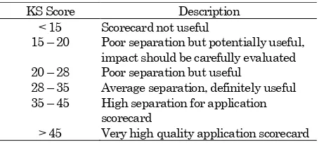
Table 3. Rules of quality assessment by
Kolmogorov-Smirnov
KS Score Description
< 15 Scorecard not useful
15 – 20 Poor separation but potentially useful, impact should be carefully evaluated 20 – 28 Poor separation but useful
28 – 35 Average separation, definitely useful 35 – 45 High separation for application
scorecard
Table 4. Weight contribution of each factor from CSM
Variable Coefficient Re-scale
score Interpretation Intercept 4.69
X5 -2.20 13.14 If there is many number
of X5 in the company, then the score is reward-ed.
X8 -0.77 4.58 If there is a person in management team beco-mes part of X8, then the score is rewarded.
X11 -1.23 7.33 If the company has more
number of X11, then the score is rewarded.
X15 -0.76 4.57 If the company business
has dependency to many of X15, then the score is rewarded.
X16 -1.83 10.95 If the company business has dependency to many of X16, then the score is rewarded.
X22 -0.62 3.70 If the currency of is match while running the busi-ness, then the score is rewarded.
X24 -4.91 29.31 If the business is owned by the company, then the score is rewarded. X28 -2.02 12.05 If the business growth
higher, then the higher score will be rewarded. X35 -0.69 4.11 If the X35 value is higher
than the upper limit, then higher score will be rewarded.
X37 -1.72 10.26 If the X37 value is higher than the upper limit, then higher score will be rewarded.
Total 100
The contribution score for each group risk factor can been seen in Table 5.
From credit scorecard above, then the observation that can be made as follows: (a) All 10 characteristics have a significant impact on the credit score at level 0.05. The highest weight is variable X24 which reflects the business condition of the client. The lowest weight is variable X22 which only contributes for 3.70% of total. (b) The business risk factors hold a major contribution for the credit score. The weight for this group is about 60.57% of total. (c) The variable X24 contributes about 29.31% of total of the credit score which dominates almost 50% in business risk factors. (d) The quality management which indicates a clear and healthy team management of the client contributes about 25.06% of total score.
Table 5. Contribution credit score per group risk factor
Charac-teristic Weight
Group risk factors
Contribution per group risk factor
X5 13.14 Quality of
management (moral risk)
25.06
X8 4.58
X11 7.33
X15 4.57
Business risk 60.57
X16 10.95
X22 3.70
X24 29.31
X28 12.05
X35 4.11
Financial risk 14.37
X37 10.26
Total 100 100
Table 6. The cut-off rates of model
Score Description
<= 20 The applicant is likely to default
21 – 65
The Credit Committee should look into the provided information for determining the creditworthiness of the applicant. >= 66 The applicant is not likely to default.
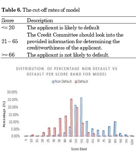
Figure 1. The distribution of the percentage of credit score
for Model 1
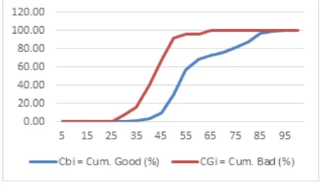
Figure 2. GINI coefficient graph model
Figure 3. Kolmogorov-Smirnov graph model
The business condition of the applicant contributes higher score for predicting the PD than the payment behavior of the applicant.
Score Distribution
After building a credit score card, it is likely to know the score distribution using the credit risk Model. The score distribution is calculated using the credit risk Model for 3818 historical loan application can be seen in Figure 1.
The observation result of Figure 1 is as follows: The distribution of default and non default applicants are clearly separated. The distribution of default appli-cants falls in the lower score and the distribution of non-default applicants falls in the higher score. There is an overlap in the score range 21 to 65. The average score of default applicants is 40.63 and the average of non-default applicants is 58.50.
Cut-off Rates
This section is to determine the cut-off rates for the scorecard. Cut-off rate is the limitation to decide whether the applicant is worth to get the loan. Based on the previous observation then the cut-off rate is given in Table 6.
Model Validation
The credit scorecard should be validated to measure its performance. The validation is using the hold 20% sample of total. The validation will include the measurement of discriminatory power and the stability population of the scorecard.
Discriminatory Power
The purpose of this test is to measure the capability of the scorecard to discrimate between default and non default applicants. There are two statistical test that can be carried out to assess the quality of the scorecard for separate “good” and “bad” customer, GINI Coefficient and KS test.
GINI Coefficient
The GINI cofficient for credit risk Model using 765 historical loan application can be seen in Figure 2. Plotting the cumulative percentages of good and bad customers per score band against each other results in the Lorenz curve. The GINI coefficient is the area between the Lorenz curve and the line indicating no separation (AC from coordinate [0,0] to [100,100]) divided by the area of the triangle ABC (B having coordinate [0,100]).
The bigger the area between the diagonal and the Lorenz curve is, the higher the efficiency of the score. Extreme values would be equal to 0, if in every score band the percentage of all bad customers is equal to the percentage of all good customers. It would be equal to 1, if a score band exists in which 100% of the bad customers lie and 0% of the good customers. If the Lorenz curve is getting closer to the A line, it indicates that there is no differences between the concentration of bad customer and good customer on same score band.
Kolmogorov-Smirnov Test
In general, the score distribution of the good custo-mers differs statistically significantly from the score distribution of the bad customers if the KS is greater than the according critical value (Figure 3). Extreme values would be:
a. 0, if in every score band the percentage of all bad customers is equal to the percentage of all good customers.
b. 1, if a score band exists in which 100% of the bad customers lie and 0% of the good customers. The graph shows that there is a gap between the score distribution of bad customer and good custo-mer. It indicates that there is a clearly separation between both of them.
Stability Population
The purpose of carry out the stability population test is to determine whether there is any difference of score distribution between the standard population (or population of the development sample) and the observed population (or population of validation sample). There are two statistical goodness-of-fit tests that can be used for measure how well the model fits to the observed population, KS and Chi-squared goodness-of-fit.
the distribution of standard population. The test statistical is lower than the critical value (1.09 < 4.92). This means that the score distribution of the observed population does not different from the standard population. Both of them come from the same distribution.
The Chi-square goodness-of-fit is carried out to test if the observed came from population with specific distribution by comparing the actual frequency with the expected frequency that would be occurred in a specific distribution for each score band. It also to test if it can be applied to binned data. If the test statistical > critical value then the distribution of observed sample is different with the distribution of standard population. The test statistical is lower than the critical value (26.78 < 30.14) with level of significant 0.05. This means that the score distri-bution of the observed population does not different significantly from the standard population. Both of them came from same distribution.
The Chi-square goodness-of-fit is carried out to test if the observed came from population with specific distribution by comparing the actual frequency with the expected frequency that would be occurred in a specific distribution for each score band. If the test statistical > critical value then the distribution of observed sample is different with the distribution of standard population. The test statistical is lower than the critical value (3.50 < 30.14) with level of significant 0.05. This means that the score distri-bution of the observed population does not different significantly from the standard population. Both of them came from same distribution.
Conclusion
In this work we developed credit-scoring model. That model contains 12 risk factors. Its performance is measured using 3,848 data application that has been scored by the model. The score distribution shows between default applicants and non-default appli-cants are clearly separated and the model can be used in the daily basis of a bank.
References
1. Thomas, L. C., Edelman, D. B., and Crook, J. N.,
Credit Scoring and Its Applications. Phila-delphia: Society for Industrial and Applied Mathematics, 2006.
2. Andreeva, G. ,European Generic Scoring Models using Survival Analysis. The Journal of the Operational Research Society, 57(10), 2006, pp. 1180–1187.
3. Andreeva, G., Ansell, J., and Crook, J. N., Credit Scoring in the Context of the European Integra-tion: Assessing the Performance of the Generic Models. Working paper. Edinburgh: Credit Research Centre, University of Edinburgh, 2008. 4. Credit Research, Rules Based Credit Scoring Methodology, Credit Research Foundation Pro-perty, 1999.
5. Thomas, L. C., Financial Risk Management Models. Risk Analysis, Assessment and Mana-gement, 1992., pp. 55–70.
6. Agresti, A., Categorical Data Analysis, John Wiley & Sons. Inc., New Jersey, USA, 2002. 7. Rossi, P. E., Allenby G. M., and McCulloch, R.,
Bayesian Statistics and Marketing, John Wiley & Sons. Inc.,West Sussex, UK., 2005.
8. R-project, www.r-project.org, 2014.
9. Robert, C., and Casella,G., Monte Carlo Statis-tical Methods (2nd edn). Springer-Verlag. New
York, 2004.
10. Hendrickx ,J., Belzer,B., Grotenhuis, M.T., and, Lammers, J., Collinearity Involving Ordered and Unordered Categorical Variables, RC33 conference in Amsterdam 2004.
http://www.xs4all.nl/~jhcjx/perturb/perturb.pdf 11. Fox, J., and Monette, G., Generalized
Collineari-ty Diagnostics, Journal of the American Statisti-cal Association; 87(417), 1992, pp. 178–183 12. Sabato, G., Assessing the Quality of Retail