THIRD EDITION
Hadoop: The Definitive Guide
Hadoop: The Definitive Guide, Third Edition by Tom White
Revision History for the :
2012-01-27 Early release revision 1
See http://oreilly.com/catalog/errata.csp?isbn=9781449311520 for release details.
Table of Contents
Foreword . . . xiii
Preface . . . xv
1. Meet Hadoop . . . 1
Data! 1
Data Storage and Analysis 3
Comparison with Other Systems 4
RDBMS 4
Grid Computing 6
Volunteer Computing 8
A Brief History of Hadoop 9
Apache Hadoop and the Hadoop Ecosystem 12
Hadoop Releases 13
What’s Covered in this Book 14
Compatibility 15
2. MapReduce . . . 17
A Weather Dataset 17
Data Format 17
Analyzing the Data with Unix Tools 19
Analyzing the Data with Hadoop 20
Map and Reduce 20
Java MapReduce 22
Scaling Out 30
Data Flow 31
Combiner Functions 34
Running a Distributed MapReduce Job 37
Hadoop Streaming 37
Ruby 37
Hadoop Pipes 41
Compiling and Running 42
3. The Hadoop Distributed Filesystem . . . 45
The Design of HDFS 45
HDFS Concepts 47
Blocks 47
Namenodes and Datanodes 48
HDFS Federation 49
HDFS High-Availability 50
The Command-Line Interface 51
Basic Filesystem Operations 52
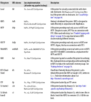
Hadoop Filesystems 54
Interfaces 55
The Java Interface 57
Reading Data from a Hadoop URL 57
Reading Data Using the FileSystem API 59
Writing Data 62
Directories 64
Querying the Filesystem 64
Deleting Data 69
Data Flow 69
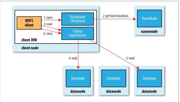
Anatomy of a File Read 69
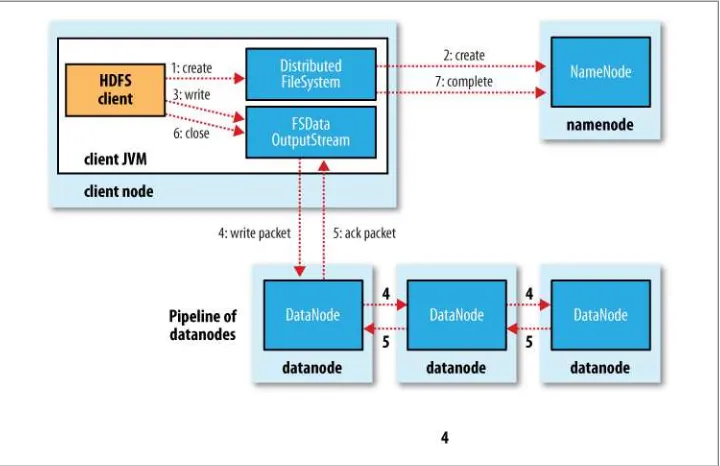
Anatomy of a File Write 72
Coherency Model 75
Parallel Copying with distcp 76
Keeping an HDFS Cluster Balanced 78
Hadoop Archives 78
Using Hadoop Archives 79
Limitations 80
4. Hadoop I/O . . . 83
Data Integrity 83
Data Integrity in HDFS 83
LocalFileSystem 84
ChecksumFileSystem 85
Compression 85
Codecs 87
Compression and Input Splits 91
Using Compression in MapReduce 92
Serialization 94
The Writable Interface 95
Implementing a Custom Writable 105
Serialization Frameworks 110
Avro 112
File-Based Data Structures 132
SequenceFile 132
MapFile 139
5. Developing a MapReduce Application . . . 145
The Configuration API 146
Combining Resources 147
Variable Expansion 148
Configuring the Development Environment 148
Managing Configuration 148
GenericOptionsParser, Tool, and ToolRunner 151
Writing a Unit Test 154
Mapper 154
Reducer 156
Running Locally on Test Data 157
Running a Job in a Local Job Runner 157
Testing the Driver 161
Running on a Cluster 162
Packaging 162
Launching a Job 162
The MapReduce Web UI 164
Retrieving the Results 167
Debugging a Job 169
Hadoop Logs 173
Remote Debugging 175
Tuning a Job 176
Profiling Tasks 177
MapReduce Workflows 180
Decomposing a Problem into MapReduce Jobs 180
JobControl 182
Apache Oozie 182
6. How MapReduce Works . . . 187
Anatomy of a MapReduce Job Run 187
Classic MapReduce (MapReduce 1) 188
YARN (MapReduce 2) 194
Failures 200
Failures in Classic MapReduce 200
Failures in YARN 202
The Fair Scheduler 205
The Capacity Scheduler 205
Shuffle and Sort 205
The Map Side 206
The Reduce Side 207
Configuration Tuning 209
Task Execution 212
The Task Execution Environment 212
Speculative Execution 213
Output Committers 215
Task JVM Reuse 216
Skipping Bad Records 217
7. MapReduce Types and Formats . . . 221
MapReduce Types 221
The Default MapReduce Job 225
Input Formats 232
Input Splits and Records 232
Text Input 243
Binary Input 247
Multiple Inputs 248
Database Input (and Output) 249
Output Formats 249
Text Output 250
Binary Output 251
Multiple Outputs 251
Lazy Output 255
Database Output 256
8. MapReduce Features . . . 257
Counters 257
Built-in Counters 257
User-Defined Java Counters 262
User-Defined Streaming Counters 266
Sorting 266
Preparation 266
Partial Sort 268
Total Sort 272
Secondary Sort 276
Joins 281
Map-Side Joins 282
Reduce-Side Joins 284
Using the Job Configuration 287
Distributed Cache 288
MapReduce Library Classes 294
9. Setting Up a Hadoop Cluster . . . 295
Cluster Specification 295
Network Topology 297
Cluster Setup and Installation 299
Installing Java 300
Creating a Hadoop User 300
Installing Hadoop 300
Testing the Installation 301
SSH Configuration 301
Hadoop Configuration 302
Configuration Management 303
Environment Settings 305
Important Hadoop Daemon Properties 309
Hadoop Daemon Addresses and Ports 314
Other Hadoop Properties 315
User Account Creation 318
YARN Configuration 318
Important YARN Daemon Properties 319
YARN Daemon Addresses and Ports 322
Security 323
Kerberos and Hadoop 324
Delegation Tokens 326
Other Security Enhancements 327
Benchmarking a Hadoop Cluster 329
Hadoop Benchmarks 329
User Jobs 331
Hadoop in the Cloud 332
Hadoop on Amazon EC2 332
10. Administering Hadoop . . . 337
HDFS 337
Persistent Data Structures 337
Safe Mode 342
Audit Logging 344
Tools 344
Monitoring 349
Logging 349
Metrics 350
Maintenance 355
Routine Administration Procedures 355
Commissioning and Decommissioning Nodes 357
Upgrades 360
11. Pig . . . 365
Installing and Running Pig 366
Execution Types 366
Running Pig Programs 368
Grunt 368
Pig Latin Editors 369
An Example 369
Generating Examples 371
Comparison with Databases 372
Pig Latin 373
Structure 373
Statements 375
Expressions 379
Types 380
Schemas 382
Functions 386
Macros 388
User-Defined Functions 389
A Filter UDF 389
An Eval UDF 392
A Load UDF 394
Data Processing Operators 397
Loading and Storing Data 397
Filtering Data 397
Grouping and Joining Data 400
Sorting Data 405
Combining and Splitting Data 406
Pig in Practice 407
Parallelism 407
Parameter Substitution 408
12. Hive . . . 411
Installing Hive 412
The Hive Shell 413
An Example 414
Running Hive 415
Configuring Hive 415
The Metastore 419
Comparison with Traditional Databases 421
Schema on Read Versus Schema on Write 421
Updates, Transactions, and Indexes 422
HiveQL 422
Data Types 424
Operators and Functions 426
Tables 427
Managed Tables and External Tables 427
Partitions and Buckets 429
Storage Formats 433
Importing Data 438
Altering Tables 440
Dropping Tables 441
Querying Data 441
Sorting and Aggregating 441
MapReduce Scripts 442
Joins 443
Subqueries 446
Views 447
User-Defined Functions 448
Writing a UDF 449
Writing a UDAF 451
13. HBase . . . 457
HBasics 457
Backdrop 458
Concepts 458
Whirlwind Tour of the Data Model 458
Implementation 459
Installation 462
Test Drive 463
Clients 465
Java 465
Avro, REST, and Thrift 468
Example 469
Schemas 470
Loading Data 471
Web Queries 474
HBase Versus RDBMS 477
Successful Service 478
HBase 479
Praxis 481
Versions 481
HDFS 482
UI 483
Metrics 483
Schema Design 483
Counters 484
Bulk Load 484
14. ZooKeeper . . . 487
Installing and Running ZooKeeper 488
An Example 490
Group Membership in ZooKeeper 490
Creating the Group 491
Joining a Group 493
Listing Members in a Group 494
Deleting a Group 496
The ZooKeeper Service 497
Data Model 497
Operations 499
Implementation 503
Consistency 505
Sessions 507
States 509
Building Applications with ZooKeeper 510
A Configuration Service 510
The Resilient ZooKeeper Application 513
A Lock Service 517
More Distributed Data Structures and Protocols 519
ZooKeeper in Production 520
Resilience and Performance 521
Configuration 522
15. Sqoop . . . 525
Getting Sqoop 525
A Sample Import 527
Generated Code 530
Additional Serialization Systems 531
Database Imports: A Deeper Look 531
Controlling the Import 534
Imports and Consistency 534
Direct-mode Imports 534
Imported Data and Hive 536
Importing Large Objects 538
Performing an Export 540
Exports: A Deeper Look 541
Exports and Transactionality 543
Exports and SequenceFiles 543
16. Case Studies . . . 545
Hadoop Usage at Last.fm 545
Last.fm: The Social Music Revolution 545
Hadoop at Last.fm 545
Generating Charts with Hadoop 546
The Track Statistics Program 547
Summary 554
Hadoop and Hive at Facebook 554
Introduction 554
Hadoop at Facebook 554
Hypothetical Use Case Studies 557
Hive 560
Problems and Future Work 564
Nutch Search Engine 565
Background 565
Data Structures 566
Selected Examples of Hadoop Data Processing in Nutch 569
Summary 578
Log Processing at Rackspace 579
Requirements/The Problem 579
Brief History 580
Choosing Hadoop 580
Collection and Storage 580
MapReduce for Logs 581
Cascading 587
Fields, Tuples, and Pipes 588
Operations 590
Taps, Schemes, and Flows 592
Cascading in Practice 593
Flexibility 596
Hadoop and Cascading at ShareThis 597
Summary 600
TeraByte Sort on Apache Hadoop 601
Using Pig and Wukong to Explore Billion-edge Network Graphs 604
Measuring Community 606
Symmetric Links 609
Community Extraction 610
A. Installing Apache Hadoop . . . 613
B. Cloudera’s Distribution for Hadoop . . . 619
Foreword
Hadoop got its start in Nutch. A few of us were attempting to build an open source web search engine and having trouble managing computations running on even a handful of computers. Once Google published its GFS and MapReduce papers, the route became clear. They’d devised systems to solve precisely the problems we were having with Nutch. So we started, two of us, half-time, to try to re-create these systems as a part of Nutch.
We managed to get Nutch limping along on 20 machines, but it soon became clear that to handle the Web’s massive scale, we’d need to run it on thousands of machines and, moreover, that the job was bigger than two half-time developers could handle. Around that time, Yahoo! got interested, and quickly put together a team that I joined. We split off the distributed computing part of Nutch, naming it Hadoop. With the help of Yahoo!, Hadoop soon grew into a technology that could truly scale to the Web. In 2006, Tom White started contributing to Hadoop. I already knew Tom through an excellent article he’d written about Nutch, so I knew he could present complex ideas in clear prose. I soon learned that he could also develop software that was as pleasant to read as his prose.
From the beginning, Tom’s contributions to Hadoop showed his concern for users and for the project. Unlike most open source contributors, Tom is not primarily interested in tweaking the system to better meet his own needs, but rather in making it easier for anyone to use.
Initially, Tom specialized in making Hadoop run well on Amazon’s EC2 and S3 serv-ices. Then he moved on to tackle a wide variety of problems, including improving the MapReduce APIs, enhancing the website, and devising an object serialization frame-work. In all cases, Tom presented his ideas precisely. In short order, Tom earned the role of Hadoop committer and soon thereafter became a member of the Hadoop Project Management Committee.
Given this, I was very pleased when I learned that Tom intended to write a book about Hadoop. Who could be better qualified? Now you have the opportunity to learn about Hadoop from a master—not only of the technology, but also of common sense and plain talk.
Preface
Martin Gardner, the mathematics and science writer, once said in an interview:
Beyond calculus, I am lost. That was the secret of my column’s success. It took me so long to understand what I was writing about that I knew how to write in a way most readers would understand.1
In many ways, this is how I feel about Hadoop. Its inner workings are complex, resting as they do on a mixture of distributed systems theory, practical engineering, and com-mon sense. And to the uninitiated, Hadoop can appear alien.
But it doesn’t need to be like this. Stripped to its core, the tools that Hadoop provides for building distributed systems—for data storage, data analysis, and coordination— are simple. If there’s a common theme, it is about raising the level of abstraction—to create building blocks for programmers who just happen to have lots of data to store, or lots of data to analyze, or lots of machines to coordinate, and who don’t have the time, the skill, or the inclination to become distributed systems experts to build the infrastructure to handle it.
With such a simple and generally applicable feature set, it seemed obvious to me when I started using it that Hadoop deserved to be widely used. However, at the time (in early 2006), setting up, configuring, and writing programs to use Hadoop was an art. Things have certainly improved since then: there is more documentation, there are more examples, and there are thriving mailing lists to go to when you have questions. And yet the biggest hurdle for newcomers is understanding what this technology is capable of, where it excels, and how to use it. That is why I wrote this book.
The Apache Hadoop community has come a long way. Over the course of three years, the Hadoop project has blossomed and spun off half a dozen subprojects. In this time, the software has made great leaps in performance, reliability, scalability, and manage-ability. To gain even wider adoption, however, I believe we need to make Hadoop even easier to use. This will involve writing more tools; integrating with more systems; and
writing new, improved APIs. I’m looking forward to being a part of this, and I hope this book will encourage and enable others to do so, too.
Administrative Notes
During discussion of a particular Java class in the text, I often omit its package name, to reduce clutter. If you need to know which package a class is in, you can easily look it up in Hadoop’s Java API documentation for the relevant subproject, linked to from the Apache Hadoop home page at http://hadoop.apache.org/. Or if you’re using an IDE, it can help using its auto-complete mechanism.
Similarly, although it deviates from usual style guidelines, program listings that import multiple classes from the same package may use the asterisk wildcard character to save space (for example: import org.apache.hadoop.io.*).
The sample programs in this book are available for download from the website that accompanies this book: http://www.hadoopbook.com/. You will also find instructions there for obtaining the datasets that are used in examples throughout the book, as well as further notes for running the programs in the book, and links to updates, additional resources, and my blog.
What’s in This Book?
The rest of this book is organized as follows. Chapter 1 emphasizes the need for Hadoop and sketches the history of the project. Chapter 2 provides an introduction to MapReduce. Chapter 3 looks at Hadoop filesystems, and in particular HDFS, in depth. Chapter 4 covers the fundamentals of I/O in Hadoop: data integrity, compression, serialization, and file-based data structures.
The next four chapters cover MapReduce in depth. Chapter 5 goes through the practical steps needed to develop a MapReduce application. Chapter 6 looks at how MapReduce is implemented in Hadoop, from the point of view of a user. Chapter 7 is about the MapReduce programming model, and the various data formats that MapReduce can work with. Chapter 8 is on advanced MapReduce topics, including sorting and joining data.
Chapters 9 and 10 are for Hadoop administrators, and describe how to set up and maintain a Hadoop cluster running HDFS and MapReduce.
Later chapters are dedicated to projects that build on Hadoop or are related to it. Chapters 11 and 12 present Pig and Hive, which are analytics platforms built on HDFS and MapReduce, whereas Chapters 13, 14, and 15 cover HBase, ZooKeeper, and Sqoop, respectively.
What’s New in the Second Edition?
The second edition has two new chapters on Hive and Sqoop (Chapters 12 and 15), a new section covering Avro (in Chapter 4), an introduction to the new security features in Hadoop (in Chapter 9), and a new case study on analyzing massive network graphs using Hadoop (in Chapter 16).
This edition continues to describe the 0.20 release series of Apache Hadoop, since this was the latest stable release at the time of writing. New features from later releases are occasionally mentioned in the text, however, with reference to the version that they were introduced in.
Conventions Used in This Book
The following typographical conventions are used in this book:
Italic
Indicates new terms, URLs, email addresses, filenames, and file extensions.
Constant width
Used for program listings, as well as within paragraphs to refer to program elements such as variable or function names, databases, data types, environment variables, statements, and keywords.
Constant width bold
Shows commands or other text that should be typed literally by the user.
Constant width italic
Shows text that should be replaced with user-supplied values or by values deter-mined by context.
This icon signifies a tip, suggestion, or general note.
This icon indicates a warning or caution.
Using Code Examples
require permission. Answering a question by citing this book and quoting example code does not require permission. Incorporating a significant amount of example code from this book into your product’s documentation does require permission.
We appreciate, but do not require, attribution. An attribution usually includes the title, author, publisher, and ISBN. For example: “Hadoop: The Definitive Guide, Second Edition, by Tom White. Copyright 2011 Tom White, 978-1-449-38973-4.”
If you feel your use of code examples falls outside fair use or the permission given above, feel free to contact us at [email protected].
Safari® Books Online
Safari Books Online is an on-demand digital library that lets you easily search over 7,500 technology and creative reference books and videos to find the answers you need quickly.
With a subscription, you can read any page and watch any video from our library online. Read books on your cell phone and mobile devices. Access new titles before they are available for print, and get exclusive access to manuscripts in development and post feedback for the authors. Copy and paste code samples, organize your favorites, down-load chapters, bookmark key sections, create notes, print out pages, and benefit from tons of other time-saving features.
O’Reilly Media has uploaded this book to the Safari Books Online service. To have full digital access to this book and others on similar topics from O’Reilly and other pub-lishers, sign up for free at http://my.safaribooksonline.com.
How to Contact Us
Please address comments and questions concerning this book to the publisher: O’Reilly Media, Inc.
1005 Gravenstein Highway North Sebastopol, CA 95472
800-998-9938 (in the United States or Canada) 707-829-0515 (international or local)
707-829-0104 (fax)
We have a web page for this book, where we list errata, examples, and any additional information. You can access this page at:
http://oreilly.com/catalog/0636920010388/ The author also has a site for this book at:
To comment or ask technical questions about this book, send email to: [email protected]
For more information about our books, conferences, Resource Centers, and the O’Reilly Network, see our website at:
http://www.oreilly.com
Acknowledgments
I have relied on many people, both directly and indirectly, in writing this book. I would like to thank the Hadoop community, from whom I have learned, and continue to learn, a great deal.
In particular, I would like to thank Michael Stack and Jonathan Gray for writing the chapter on HBase. Also thanks go to Adrian Woodhead, Marc de Palol, Joydeep Sen Sarma, Ashish Thusoo, Andrzej Białecki, Stu Hood, Chris K. Wensel, and Owen O’Malley for contributing case studies for Chapter 16.
I would like to thank the following reviewers who contributed many helpful suggestions and improvements to my drafts: Raghu Angadi, Matt Biddulph, Christophe Bisciglia, Ryan Cox, Devaraj Das, Alex Dorman, Chris Douglas, Alan Gates, Lars George, Patrick Hunt, Aaron Kimball, Peter Krey, Hairong Kuang, Simon Maxen, Olga Natkovich, Benjamin Reed, Konstantin Shvachko, Allen Wittenauer, Matei Zaharia, and Philip Zeyliger. Ajay Anand kept the review process flowing smoothly. Philip (“flip”) Kromer kindly helped me with the NCDC weather dataset featured in the examples in this book. Special thanks to Owen O’Malley and Arun C. Murthy for explaining the intricacies of the MapReduce shuffle to me. Any errors that remain are, of course, to be laid at my door.
For the second edition, I owe a debt of gratitude for the detailed review and feedback from Jeff Bean, Doug Cutting, Glynn Durham, Alan Gates, Jeff Hammerbacher, Alex Kozlov, Ken Krugler, Jimmy Lin, Todd Lipcon, Sarah Sproehnle, Vinithra Varadhara-jan, and Ian Wrigley, as well as all the readers who submitted errata for the first edition. I would also like to thank Aaron Kimball for contributing the chapter on Sqoop, and Philip (“flip”) Kromer for the case study on graph processing.
I am particularly grateful to Doug Cutting for his encouragement, support, and friend-ship, and for contributing the foreword.
Thanks also go to the many others with whom I have had conversations or email discussions over the course of writing the book.
I am grateful to my editor, Mike Loukides, and his colleagues at O’Reilly for their help in the preparation of this book. Mike has been there throughout to answer my ques-tions, to read my first drafts, and to keep me on schedule.
CHAPTER 1
Meet Hadoop
In pioneer days they used oxen for heavy pulling, and when one ox couldn’t budge a log, they didn’t try to grow a larger ox. We shouldn’t be trying for bigger computers, but for more systems of computers.
—Grace Hopper
Data!
We live in the data age. It’s not easy to measure the total volume of data stored elec-tronically, but an IDC estimate put the size of the “digital universe” at 0.18 zettabytes in 2006, and is forecasting a tenfold growth by 2011 to 1.8 zettabytes.1 A zettabyte is 1021 bytes, or equivalently one thousand exabytes, one million petabytes, or one billion terabytes. That’s roughly the same order of magnitude as one disk drive for every person in the world.
This flood of data is coming from many sources. Consider the following:2
• The New York Stock Exchange generates about one terabyte of new trade data per day.
• Facebook hosts approximately 10 billion photos, taking up one petabyte of storage. • Ancestry.com, the genealogy site, stores around 2.5 petabytes of data.
• The Internet Archive stores around 2 petabytes of data, and is growing at a rate of 20 terabytes per month.
• The Large Hadron Collider near Geneva, Switzerland, will produce about 15 petabytes of data per year.
1. From Gantz et al., “The Diverse and Exploding Digital Universe,” March 2008 (http://www.emc.com/ collateral/analyst-reports/diverse-exploding-digital-universe.pdf).
So there’s a lot of data out there. But you are probably wondering how it affects you. Most of the data is locked up in the largest web properties (like search engines), or scientific or financial institutions, isn’t it? Does the advent of “Big Data,” as it is being called, affect smaller organizations or individuals?
I argue that it does. Take photos, for example. My wife’s grandfather was an avid photographer, and took photographs throughout his adult life. His entire corpus of medium format, slide, and 35mm film, when scanned in at high-resolution, occupies around 10 gigabytes. Compare this to the digital photos that my family took in 2008, which take up about 5 gigabytes of space. My family is producing photographic data at 35 times the rate my wife’s grandfather’s did, and the rate is increasing every year as it becomes easier to take more and more photos.
More generally, the digital streams that individuals are producing are growing apace. Microsoft Research’s MyLifeBits project gives a glimpse of archiving of personal infor-mation that may become commonplace in the near future. MyLifeBits was an experi-ment where an individual’s interactions—phone calls, emails, docuexperi-ments—were cap-tured electronically and stored for later access. The data gathered included a photo taken every minute, which resulted in an overall data volume of one gigabyte a month. When storage costs come down enough to make it feasible to store continuous audio and video, the data volume for a future MyLifeBits service will be many times that. The trend is for every individual’s data footprint to grow, but perhaps more important, the amount of data generated by machines will be even greater than that generated by people. Machine logs, RFID readers, sensor networks, vehicle GPS traces, retail transactions—all of these contribute to the growing mountain of data.
The volume of data being made publicly available increases every year, too. Organiza-tions no longer have to merely manage their own data: success in the future will be dictated to a large extent by their ability to extract value from other organizations’ data. Initiatives such as Public Data Sets on Amazon Web Services, Infochimps.org, and theinfo.org exist to foster the “information commons,” where data can be freely (or in the case of AWS, for a modest price) shared for anyone to download and analyze. Mashups between different information sources make for unexpected and hitherto unimaginable applications.
Take, for example, the Astrometry.net project, which watches the Astrometry group on Flickr for new photos of the night sky. It analyzes each image and identifies which part of the sky it is from, as well as any interesting celestial bodies, such as stars or galaxies. This project shows the kind of things that are possible when data (in this case, tagged photographic images) is made available and used for something (image analysis) that was not anticipated by the creator.
however fiendish your algorithms are, they can often be beaten simply by having more data (and a less sophisticated algorithm).3
The good news is that Big Data is here. The bad news is that we are struggling to store and analyze it.
Data Storage and Analysis
The problem is simple: while the storage capacities of hard drives have increased mas-sively over the years, access speeds—the rate at which data can be read from drives— have not kept up. One typical drive from 1990 could store 1,370 MB of data and had a transfer speed of 4.4 MB/s,4 so you could read all the data from a full drive in around five minutes. Over 20 years later, one terabyte drives are the norm, but the transfer speed is around 100 MB/s, so it takes more than two and a half hours to read all the data off the disk.
This is a long time to read all data on a single drive—and writing is even slower. The obvious way to reduce the time is to read from multiple disks at once. Imagine if we had 100 drives, each holding one hundredth of the data. Working in parallel, we could read the data in under two minutes.
Only using one hundredth of a disk may seem wasteful. But we can store one hundred datasets, each of which is one terabyte, and provide shared access to them. We can imagine that the users of such a system would be happy to share access in return for shorter analysis times, and, statistically, that their analysis jobs would be likely to be spread over time, so they wouldn’t interfere with each other too much.
There’s more to being able to read and write data in parallel to or from multiple disks, though.
The first problem to solve is hardware failure: as soon as you start using many pieces of hardware, the chance that one will fail is fairly high. A common way of avoiding data loss is through replication: redundant copies of the data are kept by the system so that in the event of failure, there is another copy available. This is how RAID works, for instance, although Hadoop’s filesystem, the Hadoop Distributed Filesystem (HDFS), takes a slightly different approach, as you shall see later.
The second problem is that most analysis tasks need to be able to combine the data in some way; data read from one disk may need to be combined with the data from any of the other 99 disks. Various distributed systems allow data to be combined from multiple sources, but doing this correctly is notoriously challenging. MapReduce pro-vides a programming model that abstracts the problem from disk reads and writes,
transforming it into a computation over sets of keys and values. We will look at the details of this model in later chapters, but the important point for the present discussion is that there are two parts to the computation, the map and the reduce, and it’s the interface between the two where the “mixing” occurs. Like HDFS, MapReduce has built-in reliability.
This, in a nutshell, is what Hadoop provides: a reliable shared storage and analysis system. The storage is provided by HDFS and analysis by MapReduce. There are other parts to Hadoop, but these capabilities are its kernel.
Comparison with Other Systems
The approach taken by MapReduce may seem like a brute-force approach. The premise is that the entire dataset—or at least a good portion of it—is processed for each query. But this is its power. MapReduce is a batch query processor, and the ability to run an ad hoc query against your whole dataset and get the results in a reasonable time is transformative. It changes the way you think about data, and unlocks data that was previously archived on tape or disk. It gives people the opportunity to innovate with data. Questions that took too long to get answered before can now be answered, which in turn leads to new questions and new insights.
For example, Mailtrust, Rackspace’s mail division, used Hadoop for processing email logs. One ad hoc query they wrote was to find the geographic distribution of their users. In their words:
This data was so useful that we’ve scheduled the MapReduce job to run monthly and we will be using this data to help us decide which Rackspace data centers to place new mail servers in as we grow.
By bringing several hundred gigabytes of data together and having the tools to analyze it, the Rackspace engineers were able to gain an understanding of the data that they otherwise would never have had, and, furthermore, they were able to use what they had learned to improve the service for their customers. You can read more about how Rackspace uses Hadoop in Chapter 16.
RDBMS
The answer to these questions comes from another trend in disk drives: seek time is improving more slowly than transfer rate. Seeking is the process of moving the disk’s head to a particular place on the disk to read or write data. It characterizes the latency of a disk operation, whereas the transfer rate corresponds to a disk’s bandwidth. If the data access pattern is dominated by seeks, it will take longer to read or write large portions of the dataset than streaming through it, which operates at the transfer rate. On the other hand, for updating a small proportion of records in a database, a tradi-tional B-Tree (the data structure used in relatradi-tional databases, which is limited by the rate it can perform seeks) works well. For updating the majority of a database, a B-Tree is less efficient than MapReduce, which uses Sort/Merge to rebuild the database. In many ways, MapReduce can be seen as a complement to an RDBMS. (The differences between the two systems are shown in Table 1-1.) MapReduce is a good fit for problems that need to analyze the whole dataset, in a batch fashion, particularly for ad hoc anal-ysis. An RDBMS is good for point queries or updates, where the dataset has been in-dexed to deliver low-latency retrieval and update times of a relatively small amount of data. MapReduce suits applications where the data is written once, and read many times, whereas a relational database is good for datasets that are continually updated.
Table 1-1. RDBMS compared to MapReduce
Traditional RDBMS MapReduce Data size Gigabytes Petabytes
Access Interactive and batch Batch
Updates Read and write many times Write once, read many times
Structure Static schema Dynamic schema
Integrity High Low
Scaling Nonlinear Linear
Relational data is often normalized to retain its integrity and remove redundancy. Normalization poses problems for MapReduce, since it makes reading a record a non-local operation, and one of the central assumptions that MapReduce makes is that it is possible to perform (high-speed) streaming reads and writes.
A web server log is a good example of a set of records that is not normalized (for ex-ample, the client hostnames are specified in full each time, even though the same client may appear many times), and this is one reason that logfiles of all kinds are particularly well-suited to analysis with MapReduce.
MapReduce is a linearly scalable programming model. The programmer writes two functions—a map function and a reduce function—each of which defines a mapping from one set of key-value pairs to another. These functions are oblivious to the size of the data or the cluster that they are operating on, so they can be used unchanged for a small dataset and for a massive one. More important, if you double the size of the input data, a job will run twice as slow. But if you also double the size of the cluster, a job will run as fast as the original one. This is not generally true of SQL queries.
Over time, however, the differences between relational databases and MapReduce sys-tems are likely to blur—both as relational databases start incorporating some of the ideas from MapReduce (such as Aster Data’s and Greenplum’s databases) and, from the other direction, as higher-level query languages built on MapReduce (such as Pig and Hive) make MapReduce systems more approachable to traditional database programmers.5
Grid Computing
The High Performance Computing (HPC) and Grid Computing communities have been doing large-scale data processing for years, using such APIs as Message Passing Interface (MPI). Broadly, the approach in HPC is to distribute the work across a cluster of machines, which access a shared filesystem, hosted by a SAN. This works well for predominantly compute-intensive jobs, but becomes a problem when nodes need to access larger data volumes (hundreds of gigabytes, the point at which MapReduce really starts to shine), since the network bandwidth is the bottleneck and compute nodes become idle.
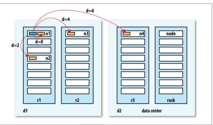
MapReduce tries to collocate the data with the compute node, so data access is fast since it is local.6 This feature, known as data locality, is at the heart of MapReduce and is the reason for its good performance. Recognizing that network bandwidth is the most precious resource in a data center environment (it is easy to saturate network links by copying data around), MapReduce implementations go to great lengths to conserve it by explicitly modelling network topology. Notice that this arrangement does not pre-clude high-CPU analyses in MapReduce.
MPI gives great control to the programmer, but requires that he or she explicitly handle the mechanics of the data flow, exposed via low-level C routines and constructs, such as sockets, as well as the higher-level algorithm for the analysis. MapReduce operates only at the higher level: the programmer thinks in terms of functions of key and value pairs, and the data flow is implicit.
Coordinating the processes in a large-scale distributed computation is a challenge. The hardest aspect is gracefully handling partial failure—when you don’t know if a remote process has failed or not—and still making progress with the overall computation. MapReduce spares the programmer from having to think about failure, since the implementation detects failed map or reduce tasks and reschedules replacements on machines that are healthy. MapReduce is able to do this since it is a shared-nothing
architecture, meaning that tasks have no dependence on one other. (This is a slight oversimplification, since the output from mappers is fed to the reducers, but this is under the control of the MapReduce system; in this case, it needs to take more care rerunning a failed reducer than rerunning a failed map, since it has to make sure it can retrieve the necessary map outputs, and if not, regenerate them by running the relevant maps again.) So from the programmer’s point of view, the order in which the tasks run doesn’t matter. By contrast, MPI programs have to explicitly manage their own check-pointing and recovery, which gives more control to the programmer, but makes them more difficult to write.
MapReduce might sound like quite a restrictive programming model, and in a sense it is: you are limited to key and value types that are related in specified ways, and mappers and reducers run with very limited coordination between one another (the mappers pass keys and values to reducers). A natural question to ask is: can you do anything useful or nontrivial with it?
The answer is yes. MapReduce was invented by engineers at Google as a system for building production search indexes because they found themselves solving the same problem over and over again (and MapReduce was inspired by older ideas from the functional programming, distributed computing, and database communities), but it has since been used for many other applications in many other industries. It is pleasantly surprising to see the range of algorithms that can be expressed in MapReduce, from
image analysis, to graph-based problems, to machine learning algorithms.7 It can’t solve every problem, of course, but it is a general data-processing tool.
You can see a sample of some of the applications that Hadoop has been used for in Chapter 16.
Volunteer Computing
When people first hear about Hadoop and MapReduce, they often ask, “How is it different from SETI@home?” SETI, the Search for Extra-Terrestrial Intelligence, runs a project called SETI@home in which volunteers donate CPU time from their otherwise idle computers to analyze radio telescope data for signs of intelligent life outside earth. SETI@home is the most well-known of many volunteer computing projects; others in-clude the Great Internet Mersenne Prime Search (to search for large prime numbers) and Folding@home (to understand protein folding and how it relates to disease). Volunteer computing projects work by breaking the problem they are trying to solve into chunks called work units, which are sent to computers around the world to be analyzed. For example, a SETI@home work unit is about 0.35 MB of radio telescope data, and takes hours or days to analyze on a typical home computer. When the analysis is completed, the results are sent back to the server, and the client gets another work unit. As a precaution to combat cheating, each work unit is sent to three different machines and needs at least two results to agree to be accepted.
Although SETI@home may be superficially similar to MapReduce (breaking a problem into independent pieces to be worked on in parallel), there are some significant differ-ences. The SETI@home problem is very CPU-intensive, which makes it suitable for running on hundreds of thousands of computers across the world,8 since the time to transfer the work unit is dwarfed by the time to run the computation on it. Volunteers are donating CPU cycles, not bandwidth.
MapReduce is designed to run jobs that last minutes or hours on trusted, dedicated hardware running in a single data center with very high aggregate bandwidth inter-connects. By contrast, SETI@home runs a perpetual computation on untrusted machines on the Internet with highly variable connection speeds and no data locality.
7. Apache Mahout (http://mahout.apache.org/) is a project to build machine learning libraries (such as classification and clustering algorithms) that run on Hadoop.
A Brief History of Hadoop
Hadoop was created by Doug Cutting, the creator of Apache Lucene, the widely used text search library. Hadoop has its origins in Apache Nutch, an open source web search engine, itself a part of the Lucene project.
The Origin of the Name “Hadoop”
The name Hadoop is not an acronym; it’s a made-up name. The project’s creator, Doug Cutting, explains how the name came about:
The name my kid gave a stuffed yellow elephant. Short, relatively easy to spell and pronounce, meaningless, and not used elsewhere: those are my naming criteria. Kids are good at generating such. Googol is a kid’s term.
Subprojects and “contrib” modules in Hadoop also tend to have names that are unre-lated to their function, often with an elephant or other animal theme (“Pig,” for example). Smaller components are given more descriptive (and therefore more mun-dane) names. This is a good principle, as it means you can generally work out what something does from its name. For example, the jobtracker9 keeps track of MapReduce
jobs.
Building a web search engine from scratch was an ambitious goal, for not only is the software required to crawl and index websites complex to write, but it is also a challenge to run without a dedicated operations team, since there are so many moving parts. It’s expensive, too: Mike Cafarella and Doug Cutting estimated a system supporting a 1-billion-page index would cost around half a million dollars in hardware, with a monthly running cost of $30,000.10 Nevertheless, they believed it was a worthy goal, as it would open up and ultimately democratize search engine algorithms.
Nutch was started in 2002, and a working crawler and search system quickly emerged. However, they realized that their architecture wouldn’t scale to the billions of pages on the Web. Help was at hand with the publication of a paper in 2003 that described the architecture of Google’s distributed filesystem, called GFS, which was being used in production at Google.11 GFS, or something like it, would solve their storage needs for the very large files generated as a part of the web crawl and indexing process. In par-ticular, GFS would free up time being spent on administrative tasks such as managing storage nodes. In 2004, they set about writing an open source implementation, the Nutch Distributed Filesystem (NDFS).
9. In this book, we use the lowercase form, “jobtracker,” to denote the entity when it’s being referred to generally, and the CamelCase form JobTracker to denote the Java class that implements it.
10. Mike Cafarella and Doug Cutting, “Building Nutch: Open Source Search,” ACM Queue, April 2004, http: //queue.acm.org/detail.cfm?id=988408.
In 2004, Google published the paper that introduced MapReduce to the world.12 Early in 2005, the Nutch developers had a working MapReduce implementation in Nutch, and by the middle of that year all the major Nutch algorithms had been ported to run using MapReduce and NDFS.
NDFS and the MapReduce implementation in Nutch were applicable beyond the realm of search, and in February 2006 they moved out of Nutch to form an independent subproject of Lucene called Hadoop. At around the same time, Doug Cutting joined Yahoo!, which provided a dedicated team and the resources to turn Hadoop into a system that ran at web scale (see sidebar). This was demonstrated in February 2008 when Yahoo! announced that its production search index was being generated by a 10,000-core Hadoop cluster.13
In January 2008, Hadoop was made its own top-level project at Apache, confirming its success and its diverse, active community. By this time, Hadoop was being used by many other companies besides Yahoo!, such as Last.fm, Facebook, and the New York Times. Some applications are covered in the case studies in Chapter 16 and on the Hadoop wiki.
In one well-publicized feat, the New York Times used Amazon’s EC2 compute cloud to crunch through four terabytes of scanned archives from the paper converting them to PDFs for the Web.14 The processing took less than 24 hours to run using 100 ma-chines, and the project probably wouldn’t have been embarked on without the com-bination of Amazon’s pay-by-the-hour model (which allowed the NYT to access a large number of machines for a short period) and Hadoop’s easy-to-use parallel program-ming model.
In April 2008, Hadoop broke a world record to become the fastest system to sort a terabyte of data. Running on a 910-node cluster, Hadoop sorted one terabyte in 209 seconds (just under 3½ minutes), beating the previous year’s winner of 297 seconds (described in detail in “TeraByte Sort on Apache Hadoop” on page 601). In November of the same year, Google reported that its MapReduce implementation sorted one ter-abyte in 68 seconds.15 As the first edition of this book was going to press (May 2009), it was announced that a team at Yahoo! used Hadoop to sort one terabyte in 62 seconds.
12. Jeffrey Dean and Sanjay Ghemawat, “MapReduce: Simplified Data Processing on Large Clusters ,” December 2004, http://labs.google.com/papers/mapreduce.html.
13. “Yahoo! Launches World’s Largest Hadoop Production Application,” 19 February 2008, http://developer .yahoo.net/blogs/hadoop/2008/02/yahoo-worlds-largest-production-hadoop.html.
14. Derek Gottfrid, “Self-service, Prorated Super Computing Fun!” 1 November 2007, http://open.blogs .nytimes.com/2007/11/01/self-service-prorated-super-computing-fun/.
Hadoop at Yahoo!
Building Internet-scale search engines requires huge amounts of data and therefore large numbers of machines to process it. Yahoo! Search consists of four primary com-ponents: the Crawler, which downloads pages from web servers; the WebMap, which builds a graph of the known Web; the Indexer, which builds a reverse index to the best pages; and the Runtime, which answers users’ queries. The WebMap is a graph that consists of roughly 1 trillion (1012) edges each representing a web link and 100 billion
(1011) nodes each representing distinct URLs. Creating and analyzing such a large graph
requires a large number of computers running for many days. In early 2005, the infra-structure for the WebMap, named Dreadnaught, needed to be redesigned to scale up to more nodes. Dreadnaught had successfully scaled from 20 to 600 nodes, but required a complete redesign to scale out further. Dreadnaught is similar to MapReduce in many ways, but provides more flexibility and less structure. In particular, each fragment in a Dreadnaught job can send output to each of the fragments in the next stage of the job, but the sort was all done in library code. In practice, most of the WebMap phases were pairs that corresponded to MapReduce. Therefore, the WebMap applications would not require extensive refactoring to fit into MapReduce.
Eric Baldeschwieler (Eric14) created a small team and we started designing and prototyping a new framework written in C++ modeled after GFS and MapReduce to replace Dreadnaught. Although the immediate need was for a new framework for WebMap, it was clear that standardization of the batch platform across Yahoo! Search was critical and by making the framework general enough to support other users, we could better leverage investment in the new platform.
At the same time, we were watching Hadoop, which was part of Nutch, and its progress. In January 2006, Yahoo! hired Doug Cutting, and a month later we decided to abandon our prototype and adopt Hadoop. The advantage of Hadoop over our prototype and design was that it was already working with a real application (Nutch) on 20 nodes. That allowed us to bring up a research cluster two months later and start helping real customers use the new framework much sooner than we could have otherwise. Another advantage, of course, was that since Hadoop was already open source, it was easier (although far from easy!) to get permission from Yahoo!’s legal department to work in open source. So we set up a 200-node cluster for the researchers in early 2006 and put the WebMap conversion plans on hold while we supported and improved Hadoop for the research users.
Here’s a quick timeline of how things have progressed:
• 2004—Initial versions of what is now Hadoop Distributed Filesystem and Map-Reduce implemented by Doug Cutting and Mike Cafarella.
• December 2005—Nutch ported to the new framework. Hadoop runs reliably on 20 nodes.
• January 2006—Doug Cutting joins Yahoo!.
• February 2006—Adoption of Hadoop by Yahoo! Grid team.
• April 2006—Sort benchmark (10 GB/node) run on 188 nodes in 47.9 hours. • May 2006—Yahoo! set up a Hadoop research cluster—300 nodes.
• May 2006—Sort benchmark run on 500 nodes in 42 hours (better hardware than April benchmark).
• October 2006—Research cluster reaches 600 nodes.
• December 2006—Sort benchmark run on 20 nodes in 1.8 hours, 100 nodes in 3.3 hours, 500 nodes in 5.2 hours, 900 nodes in 7.8 hours.
• January 2007—Research cluster reaches 900 nodes. • April 2007—Research clusters—2 clusters of 1000 nodes.
• April 2008—Won the 1 terabyte sort benchmark in 209 seconds on 900 nodes. • October 2008—Loading 10 terabytes of data per day on to research clusters. • March 2009—17 clusters with a total of 24,000 nodes.
• April 2009—Won the minute sort by sorting 500 GB in 59 seconds (on 1,400 nodes) and the 100 terabyte sort in 173 minutes (on 3,400 nodes).
—Owen O’Malley
Apache Hadoop and the Hadoop Ecosystem
Although Hadoop is best known for MapReduce and its distributed filesystem (HDFS, renamed from NDFS), the term is also used for a family of related projects that fall under the umbrella of infrastructure for distributed computing and large-scale data processing.
All of the core projects covered in this book are hosted by the Apache Software Foun-dation, which provides support for a community of open source software projects, including the original HTTP Server from which it gets its name. As the Hadoop eco-system grows, more projects are appearing, not necessarily hosted at Apache, which provide complementary services to Hadoop, or build on the core to add higher-level abstractions.
The Hadoop projects that are covered in this book are described briefly here:
Common
A set of components and interfaces for distributed filesystems and general I/O (serialization, Java RPC, persistent data structures).
Avro
A serialization system for efficient, cross-language RPC, and persistent data storage.
MapReduce
HDFS
A distributed filesystem that runs on large clusters of commodity machines.
Pig
A data flow language and execution environment for exploring very large datasets. Pig runs on HDFS and MapReduce clusters.
Hive
A distributed data warehouse. Hive manages data stored in HDFS and provides a query language based on SQL (and which is translated by the runtime engine to MapReduce jobs) for querying the data.
HBase
A distributed, column-oriented database. HBase uses HDFS for its underlying storage, and supports both batch-style computations using MapReduce and point queries (random reads).
ZooKeeper
A distributed, highly available coordination service. ZooKeeper provides primitives such as distributed locks that can be used for building distributed applications.
Sqoop
A tool for efficiently moving data between relational databases and HDFS.
Hadoop Releases
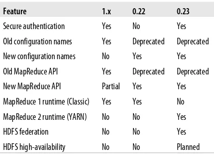
Which version of Hadoop should you use? The answer to this question changes over time, of course, and also depends on the features that you need. “Hadoop Relea-ses” on page 13 summarizes the high-level features in recent Hadoop release series. There are a few active release series. The 1.x release series is a continuation of the 0.20 release series, and contains the most stable versions of Hadoop currently available. This series includes secure Kerberos authentication, which prevents unauthorized access to Hadoop data (see “Security” on page 323). Almost all production clusters use these releases, or derived versions (such as commercial distributions).
The 0.22 and 0.23 release series16 are currently marked as alpha releases (as of early 2012), but this is likely to change by the time you read this as they get more real-world testing and become more stable (consult the Apache Hadoop releases page for the latest status). 0.23 includes several major new features:
• A new MapReduce runtime, called MapReduce 2, implemented on a new system called YARN (Yet Another Resource Negotiator), which is a general resource man-agement system for running distributed applications. MapReduce 2 replaces the
“classic” runtime in previous releases. It is described in more depth in “YARN (MapReduce 2)” on page 194.
• HDFS federation, which partitions the HDFS namespace across multiple namen-odes to support clusters with very large numbers of files. See “HDFS Federa-tion” on page 49.
• HDFS high-availability, which removes the namenode as a single point of failure by supporting standby namenodes for failover. See “HDFS High-Availabil-ity” on page 50.
Table 1-2. Features Supported by Hadoop Release Series
Feature 1.x 0.22 0.23
Secure authentication Yes No Yes
Old configuration names Yes Deprecated Deprecated
New configuration names No Yes Yes
Old MapReduce API Yes Deprecated Deprecated
New MapReduce API Partial Yes Yes
MapReduce 1 runtime (Classic) Yes Yes No
MapReduce 2 runtime (YARN) No No Yes
HDFS federation No No Yes
HDFS high-availability No No Planned
Table 1-2 only covers features in HDFS and MapReduce. Other projects in the Hadoop ecosystem are continually evolving too, and picking a combination of components that work well together can be a challenge. Thankfully, you don’t have to do this work yourself. The Apache Bigtop project (http://incubator.apache.org/bigtop/) runs intero-perability tests on stacks of Hadoop components, and provides binary packages (RPMs and Debian packages) for easy installation. There are also commercial vendors offering Hadoop distributions containing suites of compatible components.
What’s Covered in this Book
This book covers all the releases in Table 1-2. In the cases where a feature is only available in a particular release, it is noted in the text.
The code in this book is written to work against all these release series, except in a small number of cases, which are explicitly called out. The example code available on the website has a list of the versions that it was tested against.
Configuration Names
per-taining to the namenode have been changed to have a dfs.namenode prefix, so dfs.name.dir has changed to dfs.namenode.name.dir. Similarly, MapReduce properties
have the mapreduce prefix, rather than the older mapred prefix, so mapred.job.name has
changed to mapreduce.job.name.
For properties that exist in version 1.x, the old (deprecated) names are used in this book, since they will work in all the versions of Hadoop listed here. If you are using a release after 1.x, you may wish to use the new property names in your configuration files and code to remove deprecation warnings. A table listing the deprecated properties names and their replacements can be found on the Hadoop website at http://hadoop .apache.org/common/docs/r0.23.0/hadoop-project-dist/hadoop-common/Deprecated Properties.html.
MapReduce APIs
Hadoop provides two Java MapReduce APIs, described in more detail in “The old and the new Java MapReduce APIs” on page 27. This edition of the book uses the new API, which will work with all versions listed here, except in a few cases where that part of the new API is not available in the 1.x releases. In these cases the equivalent code using the old API is available on the book’s website.
Compatibility
When moving from one release to another you need to consider the upgrade steps that are needed. There are several aspects to consider: API compatibility, data compatibility, and wire compatibility.
API compatibility concerns the contract between user code and the published Hadoop APIs, such as the Java MapReduce APIs. Major releases (e.g. from 1.x.y to 2.0.0) are allowed to break API compatibility, so user programs may need to be modified and recompiled. Minor releases (e.g. from 1.0.x to 1.1.0) and point releases (e.g. from 1.0.1 to 1.0.2) should not break compatibility.17
Hadoop uses a classification scheme for API elements to denote their stability. The above rules for API compatibility cover those elements that are marked InterfaceStability.Stable. Some elements of the pub-lic Hadoop APIs, however, are marked with the InterfaceStabil ity.Evolving or InterfaceStability.Unstable annotations (all these an-notations are in the org.apache.hadoop.classification package), which means they are allowed to break compatibility on minor and point re-leases, respectively.
Data compatibility concerns persistent data and metadata formats, such as the format in which the HDFS namenode stores its persistent data. The formats can change across minor or major releases, but the change is transparent to users since the upgrade will automatically migrate the data. There may be some restrictions about upgrade paths, and these are covered in the release notes—for example it may be necessary to upgrade via an intermediate release rather than upgrading directly to the later final release in one step. Hadoop upgrades are discussed in more detail in “Upgrades” on page 360. Wire compatibility concerns the interoperability between clients and servers via wire protocols like RPC and HTTP. There are two types of client: external clients (run by users) and internal clients (run on the cluster as a part of the system, e.g. datanode and tasktracker daemons). In general, internal clients have to be upgraded in lockstep—an older version of a tasktracker will not work with a newer jobtracker, for example. In the future rolling upgrades may be supported, which would allow cluster daemons to be upgraded in phases, so that the cluster would still be available to external clients during the upgrade.
CHAPTER 2
MapReduce
MapReduce is a programming model for data processing. The model is simple, yet not too simple to express useful programs in. Hadoop can run MapReduce programs writ-ten in various languages; in this chapter, we shall look at the same program expressed in Java, Ruby, Python, and C++. Most important, MapReduce programs are inherently parallel, thus putting very large-scale data analysis into the hands of anyone with enough machines at their disposal. MapReduce comes into its own for large datasets, so let’s start by looking at one.
A Weather Dataset
For our example, we will write a program that mines weather data. Weather sensors collecting data every hour at many locations across the globe gather a large volume of log data, which is a good candidate for analysis with MapReduce, since it is semi-structured and record-oriented.
Data Format
Example 2-1. Format of a National Climate Data Center record
0057
332130 # USAF weather station identifier 99999 # WBAN weather station identifier 19500101 # observation date
0300 # observation time 4
+51317 # latitude (degrees x 1000) +028783 # longitude (degrees x 1000) FM-12
00450 # sky ceiling height (meters) 1 # quality code
C N
010000 # visibility distance (meters) 1 # quality code
N 9
-0128 # air temperature (degrees Celsius x 10) 1 # quality code
-0139 # dew point temperature (degrees Celsius x 10) 1 # quality code
10268 # atmospheric pressure (hectopascals x 10) 1 # quality code
Data files are organized by date and weather station. There is a directory for each year from 1901 to 2001, each containing a gzipped file for each weather station with its readings for that year. For example, here are the first entries for 1990:
% ls raw/1990 | head
year’s readings were concatenated into a single file. (The means by which this was carried out is described in Appendix C.)
Analyzing the Data with Unix Tools
What’s the highest recorded global temperature for each year in the dataset? We will answer this first without using Hadoop, as this information will provide a performance baseline, as well as a useful means to check our results.
The classic tool for processing line-oriented data is awk. Example 2-2 is a small script to calculate the maximum temperature for each year.
Example 2-2. A program for finding the maximum recorded temperature by year from NCDC weather records
#!/usr/bin/env bash for year in all/* do
echo -ne `basename $year .gz`"\t" gunzip -c $year | \
awk '{ temp = substr($0, 88, 5) + 0; q = substr($0, 93, 1);
if (temp !=9999 && q ~ /[01459]/ && temp > max) max = temp } END { print max }'
done
The script loops through the compressed year files, first printing the year, and then processing each file using awk. The awk script extracts two fields from the data: the air temperature and the quality code. The air temperature value is turned into an integer by adding 0. Next, a test is applied to see if the temperature is valid (the value 9999 signifies a missing value in the NCDC dataset) and if the quality code indicates that the reading is not suspect or erroneous. If the reading is OK, the value is compared with the maximum value seen so far, which is updated if a new maximum is found. The
END block is executed after all the lines in the file have been processed, and it prints the
maximum value.
Here is the beginning of a run: % ./max_temperature.sh 1901 317
1902 244 1903 289 1904 256 1905 283 ...
To speed up the processing, we need to run parts of the program in parallel. In theory, this is straightforward: we could process different years in different processes, using all the available hardware threads on a machine. There are a few problems with this, however.
First, dividing the work into equal-size pieces isn’t always easy or obvious. In this case, the file size for different years varies widely, so some processes will finish much earlier than others. Even if they pick up further work, the whole run is dominated by the longest file. A better approach, although one that requires more work, is to split the input into fixed-size chunks and assign each chunk to a process.
Second, combining the results from independent processes may need further process-ing. In this case, the result for each year is independent of other years and may be combined by concatenating all the results, and sorting by year. If using the fixed-size chunk approach, the combination is more delicate. For this example, data for a par-ticular year will typically be split into several chunks, each processed independently. We’ll end up with the maximum temperature for each chunk, so the final step is to look for the highest of these maximums, for each year.
Third, you are still limited by the processing capacity of a single machine. If the best time you can achieve is 20 minutes with the number of processors you have, then that’s it. You can’t make it go faster. Also, some datasets grow beyond the capacity of a single machine. When we start using multiple machines, a whole host of other factors come into play, mainly falling in the category of coordination and reliability. Who runs the overall job? How do we deal with failed processes?
So, though it’s feasible to parallelize the processing, in practice it’s messy. Using a framework like Hadoop to take care of these issues is a great help.
Analyzing the Data with Hadoop
To take advantage of the parallel processing that Hadoop provides, we need to express our query as a MapReduce job. After some local, small-scale testing, we will be able to run it on a cluster of machines.
Map and Reduce
MapReduce works by breaking the processing into two phases: the map phase and the reduce phase. Each phase has key-value pairs as input and output, the types of which may be chosen by the programmer. The programmer also specifies two functions: the map function and the reduce function.
Our map function is simple. We pull out the year and the air temperature, since these are the only fields we are interested in. In this case, the map function is just a data preparation phase, setting up the data in such a way that the reducer function can do its work on it: finding the maximum temperature for each year. The map function is also a good place to drop bad records: here we filter out temperatures that are missing, suspect, or erroneous.
To visualize the way the map works, consider the following sample lines of input data (some unused columns have been dropped to fit the page, indicated by ellipses):
0067011990999991950051507004...9999999N9+00001+99999999999... 0043011990999991950051512004...9999999N9+00221+99999999999... 0043011990999991950051518004...9999999N9-00111+99999999999... 0043012650999991949032412004...0500001N9+01111+99999999999... 0043012650999991949032418004...0500001N9+00781+99999999999...
These lines are presented to the map function as the key-value pairs: (0, 0067011990999991950051507004...9999999N9+00001+99999999999...) (106, 0043011990999991950051512004...9999999N9+00221+99999999999...) (212, 0043011990999991950051518004...9999999N9-00111+99999999999...) (318, 0043012650999991949032412004...0500001N9+01111+99999999999...) (424, 0043012650999991949032418004...0500001N9+00781+99999999999...)
The keys are the line offsets within the file, which we ignore in our map function. The map function merely extracts the year and the air temperature (indicated in bold text), and emits them as its output (the temperature values have been interpreted as integers):
(1950, 0) (1950, 22) (1950, −11) (1949, 111) (1949, 78)
The output from the map function is processed by the MapReduce framework before being sent to the reduce function. This processing sorts and groups the key-value pairs by key. So, continuing the example, our reduce function sees the following input:
(1949, [111, 78]) (1950, [0, 22, −11])
Each year appears with a list of all its air temperature readings. All the reduce function has to do now is iterate through the list and pick up the maximum reading:
(1949, 111) (1950, 22)
Java MapReduce
Having run through how the MapReduce program works, the next step is to express it in code. We need three things: a map function, a reduce function, and some code to run the job. The map function is represented by the Mapper class, which declares an
abstract map() method. Example 2-3 shows the implementation of our map method.
Example 2-3. Mapper for maximum temperature example
import java.io.IOException;
import org.apache.hadoop.io.IntWritable; import org.apache.hadoop.io.LongWritable; import org.apache.hadoop.io.Text;
import org.apache.hadoop.mapreduce.Mapper;
public class MaxTemperatureMapper
extends Mapper<LongWritable, Text, Text, IntWritable> {
private static final int MISSING = 9999;
@Override
public void map(LongWritable key, Text value, Context context) throws IOException, InterruptedException {
String line = value.toString(); String year = line.substring(15, 19); int airTemperature;
if (line.charAt(87) == '+') { // parseInt doesn't like leading plus signs airTemperature = Integer.parseInt(line.substring(88, 92));
} else {
airTemperature = Integer.parseInt(line.substring(87, 92)); }
String quality = line.substring(92, 93);
if (airTemperature != MISSING && quality.matches("[01459]")) { context.write(new Text(year), new IntWritable(airTemperature)); }
} }
The Mapper class is a generic type, with four formal type parameters that specify the