Demystified Series
Advanced Statistics Demystified Algebra Demystified
Anatomy Demystified Astronomy Demystified Biology Demystified
Business Statistics Demystified Calculus Demystified
Chemistry Demystified College Algebra Demystified Differential Equations Demystified Digital Electronics Demystified Earth Science Demystified Electricity Demystified Electronics Demystified Everyday Math Demystified Geometry Demystified
Math Word Problems Demystified Microbiology Demystified
Physics Demystified Physiology Demystified Pre-Algebra Demystified Precalculus Demystified Probability Demystified
Project Management Demystified Robotics Demystified
PROBABILITY DEMYSTIFIED
ALLAN G. BLUMAN
Copyright © 2005 by The McGraw-Hill Companies, Inc. All rights reserved. Manufactured in the United States of America. Except as permitted under the United States Copyright Act of 1976, no part of this publication may be reproduced or distributed in any form or by any means, or stored in a database or retrieval system, without the prior written permission of the publisher.
0-07-146999-0
The material in this eBook also appears in the print version of this title: 0-07-144549-8.
All trademarks are trademarks of their respective owners. Rather than put a trademark symbol after every occurrence of a trademarked name, we use names in an editorial fashion only, and to the benefit of the trademark owner, with no intention of infringement of the trademark. Where such designations appear in this book, they have been printed with initial caps. McGraw-Hill eBooks are available at special quantity discounts to use as premiums and sales promotions, or for use in corporate training programs. For more information, please contact George Hoare, Special Sales, at [email protected] or (212) 904-4069.
TERMS OF USE
This is a copyrighted work and The McGraw-Hill Companies, Inc. (“McGraw-Hill”) and its licensors reserve all rights in and to the work. Use of this work is subject to these terms. Except as permitted under the Copyright Act of 1976 and the right to store and retrieve one copy of the work, you may not decompile, disassemble, reverse engineer, reproduce, modify, create derivative works based upon, transmit, distribute, disseminate, sell, publish or sublicense the work or any part of it without McGraw-Hill’s prior consent. You may use the work for your own noncommercial and personal use; any other use of the work is strictly prohibited. Your right to use the work may be terminated if you fail to comply with these terms.
THE WORK IS PROVIDED “AS IS.” McGRAW-HILL AND ITS LICENSORS MAKE NO GUARANTEES OR WARRANTIES AS TO THE ACCURACY, ADEQUACY OR COMPLETENESS OF OR RESULTS TO BE OBTAINED FROM USING THE WORK, INCLUDING ANY INFORMATION THAT CAN BE ACCESSED THROUGH THE WORK VIA HYPERLINK OR OTHERWISE, AND EXPRESSLY DISCLAIM ANY WARRANTY, EXPRESS OR IMPLIED, INCLUDING BUT NOT LIMITED TO IMPLIED WARRANTIES OF MERCHANTABILITY OR FITNESS FOR A PARTICULAR PURPOSE. McGraw-Hill and its licensors do not warrant or guarantee that the functions contained in the work will meet your requirements or that its operation will be uninterrupted or error free. Neither McGraw-Hill nor its licensors shall be liable to you or anyone else for any inaccuracy, error or omission, regardless of cause, in the work or for any damages resulting therefrom. McGraw-Hill has no responsibility for the content of any information accessed through the work. Under no circumstances shall McGraw-Hill and/or its licensors be liable for any indirect, incidental, special, punitive, consequential or similar damages that result from the use of or inability to use the work, even if any of them has been advised of the possibility of such damages. This limitation of liability shall apply to any claim or cause whatsoever whether such claim or cause arises in contract, tort or otherwise.
������������
Want to learn more?
We hope you enjoy this
CONTENTS
Preface
ix
Acknowledgments
xi
CHAPTER 1
Basic Concepts
1
CHAPTER 2
Sample Spaces
22
CHAPTER 3
The Addition Rules
43
CHAPTER 4
The Multiplication Rules
56
CHAPTER 5
Odds and Expectation
77
CHAPTER 6
The Counting Rules
94
CHAPTER 7
The Binomial Distribution
114
CHAPTER 8
Other Probability Distributions
131
CHAPTER 9
The Normal Distribution
147
CHAPTER 10
Simulation
177
CHAPTER 11
Game Theory
187
CHAPTER 12
Actuarial Science
210
Final Exam
229
Answers to Quizzes and Final Exam
244
Appendix: Bayes’ Theorem
249
Index
255
vii
PREFACE
‘‘The probable is what usually happens.’’ — Aristotle
Probability can be called the mathematics of chance. The theory of probabil-ity is unusual in the sense that we cannot predict with certainty the individual outcome of a chance process such as flipping a coin or rolling a die (singular for dice), but we can assign a number that corresponds to the probability of getting a particular outcome. For example, the probability of getting a head when a coin is tossed is 1/2 and the probability of getting a two when a single fair die is rolled is 1/6.
We can also predict with a certain amount of accuracy that when a coin is tossed a large number of times, the ratio of the number of heads to the total number of times the coin is tossed will be close to 1/2.
Probability theory is, of course, used in gambling. Actually, mathemati-cians began studying probability as a means to answer questions about gambling games. Besides gambling, probability theory is used in many other areas such as insurance, investing, weather forecasting, genetics, and medicine, and in everyday life.
What is this book about?
First let me tell you what this book isnot about:
. This book is not a rigorous theoretical deductive mathematical approach to the concepts of probability.
. This book isnota book on how to gamble. And most important
ix
. This book isnot a book on how to win at gambling!
This book presents the basic concepts of probability in a simple, straightforward, easy-to-understand way. It does require, however, a knowledge of arithmetic (fractions, decimals, and percents) and a knowledge of basic algebra (formulas, exponents, order of operations, etc.). If you need a review of these concepts, you can consult another of my books in this series entitledPre-Algebra Demystified.
This book can be used to gain a knowledge of the basic concepts of probability theory, either as a self-study guide or as a supplementary textbook for those who are taking a course in probability or a course in statistics that has a section on probability.
The basic concepts of probability are explained in the first two chapters. Then the addition and multiplication rules are explained. Following that, the concepts of odds and expectation are explained. The counting rules are explained in Chapter 6, and they are needed for the binomial and other probability distributions found in Chapters 7 and 8. The relationship between probability and the normal distribution is presented in Chapter 9. Finally, a recent development, the Monte Carlo method of simulation, is explained in Chapter 10. Chapter 11 explains how probability can be used in game theory and Chapter 12 explains how probability is used in actuarial science. Special material on Bayes’ Theorem is presented in the Appendix because this concept is somewhat more difficult than the other concepts presented in this book.
In addition to addressing the concepts of probability, each chapter ends with what is called a ‘‘Probability Sidelight.’’ These sections cover some of the historical aspects of the development of probability theory or some commentary on how probability theory is used in gambling and everyday life. I have spent my entire career teaching mathematics at a level that most students can understand and appreciate. I have written this book with the same objective in mind. Mathematical precision, in some cases, has been sacrificed in the interest of presenting probability theory in a simplified way.
Good luck!
Allan G. Bluman
PREFACE
ACKNOWLEDGMENTS
I would like to thank my wife, Betty Claire, for helping me with the prepara-tion of this book and my editor, Judy Bass, for her assistance in its pub-lication. I would also like to thank Carrie Green for her error checking and helpful suggestions.
xi
CHAPTER
1
Basic Concepts
Introduction
Probability can be defined as the mathematics of chance. Most people are familiar with some aspects of probability by observing or playing gambling games such as lotteries, slot machines, black jack, or roulette. However, probability theory is used in many other areas such as business, insurance, weather forecasting, and in everyday life.
In this chapter, you will learn about the basic concepts of probability using various devices such as coins, cards, and dice. These devices are not used as examples in order to make you an astute gambler, but they are used because they will help you understand the concepts of probability.
1
Probability Experiments
Chance processes, such as flipping a coin, rolling a die (singular for dice), or drawing a card at random from a well-shuffled deck are called probability experiments. Aprobability experimentis a chance process that leads to well-defined outcomes or results. For example, tossing a coin can be considered a probability experiment since there are two well-defined outcomes—heads and tails.
An outcome of a probability experiment is the result of a single trial of a probability experiment. A trial means flipping a coin once, or drawing a single card from a deck. A trial could also mean rolling two dice at once, tossing three coins at once, or drawing five cards from a deck at once. A single trial of a probability experiment means to perform the experiment one time.
The set of all outcomes of a probability experiment is called a sample space. Some sample spaces for various probability experiments are shown here.
Experiment Sample Space
Toss one coin H, T* Roll a die 1, 2, 3, 4, 5, 6 Toss two coins HH, HT, TH, TT
*H = heads; T = tails.
Notice that when two coins are tossed, there are four outcomes, not three. Consider tossing a nickel and a dime at the same time. Both coins could fall heads up. Both coins could fall tails up. The nickel could fall heads up and the dime could fall tails up, or the nickel could fall tails up and the dime could fall heads up. The situation is the same even if the coins are indistinguishable.
It should be mentioned that each outcome of a probability experiment occurs at random. This means you cannot predict with certainty which outcome will occur when the experiment is conducted. Also, each outcome of the experiment is equally likelyunless otherwise stated. That means that each outcome has the same probability of occurring.
When finding probabilities, it is often necessary to consider several outcomes of the experiment. For example, when a single die is rolled, you may want to consider obtaining an even number; that is, a two, four, or six. This is called an event. An event then usually consists of one or more
CHAPTER 1
Basic Concepts
outcomes of the sample space. (Note: It is sometimes necessary to consider an event which has no outcomes. This will be explained later.)
An event with one outcome is called asimple event. For example, a die is rolled and the event of getting a four is a simple event since there is only one way to get a four. When an event consists of two or more outcomes, it is called acompound event. For example, if a die is rolled and the event is getting an odd number, the event is a compound event since there are three ways to get an odd number, namely, 1, 3, or 5.
Simple and compound events should not be confused with the number of times the experiment is repeated. For example, if two coins are tossed, the event of getting two heads is a simple event since there is only one way to get two heads, whereas the event of getting a head and a tail in either order is a compound event since it consists of two outcomes, namely head, tail and tail, head.
EXAMPLE: A single die is rolled. List the outcomes in each event: a. Getting an odd number
b. Getting a number greater than four c. Getting less than one
SOLUTION:
a. The event contains the outcomes 1, 3, and 5. b. The event contains the outcomes 5 and 6.
c. When you roll a die, you cannot get a number less than one; hence, the event contains no outcomes.
Classical Probability
Sample spaces are used in classical probability to determine the numerical probability that an event will occur. The formula for determining the probability of an event Eis
PðEÞ ¼number of outcomes contained in the event E
total number of outcomes in the sample space
EXAMPLE: Two coins are tossed; find the probability that both coins land heads up.
SOLUTION:
The sample space for tossing two coins is HH, HT, TH, and TT. Since there are 4 events in the sample space, and only one way to get two heads (HH), the answer is
PðHHÞ ¼1 4
EXAMPLE: A die is tossed; find the probability of each event: a. Getting a two
b. Getting an even number c. Getting a number less than 5
SOLUTION:
The sample space is 1, 2, 3, 4, 5, 6, so there are six outcomes in the sample space.
a. P(2)¼1
6, since there is only one way to obtain a 2. b. P(even number) ¼3
6 ¼ 1
2, since there are three ways to get an odd number, 1, 3, or 5.
c. P(number less than 5Þ ¼4 6¼
2
3, since there are four numbers in the sample space less than 5.
EXAMPLE: A dish contains 8 red jellybeans, 5 yellow jellybeans, 3 black jellybeans, and 4 pink jellybeans. If a jellybean is selected at random, find the probability that it is
a. A red jellybean
b. A black or pink jellybean c. Not yellow
d. An orange jellybean
CHAPTER 1
Basic Concepts
SOLUTION:
There are 8 + 5 + 3 + 4 = 20 outcomes in the sample space. a. PðredÞ ¼ 8
20¼ 2 5
b. Pðblack or pinkÞ ¼3þ4 20 ¼
7 20
c. P(not yellow) =P(red or black or pink)¼8þ3þ4 20 ¼
15 20¼
3 4 d. P(orange)=0
20¼0, since there are no orange jellybeans.
Probabilities can be expressed as reduced fractions, decimals, or percents. For example, if a coin is tossed, the probability of getting heads up is 1
2 or
0.5 or 50%. (Note: Some mathematicians feel that probabilities should be expressed only as fractions or decimals. However, probabilities are often given as percents in everyday life. For example, one often hears, ‘‘There is a 50% chance that it will rain tomorrow.’’)
Probability problems use a certain language. For example, suppose a die is tossed. An event that is specified as ‘‘getting at least a 3’’ means getting a 3, 4, 5, or 6. An event that is specified as ‘‘getting at most a 3’’ means getting a 1, 2, or 3.
Probability Rules
There are certain rules that apply to classical probability theory. They are presented next.
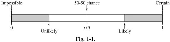
Rule 1:The probability of any event will always be a number from zero to one. This can be denoted mathematically as 0P(E)1. What this means is that all answers to probability problems will be numbers ranging from zero to one. Probabilities cannot be negative nor can they be greater than one.
Also, when the probability of an event is close to zero, the occurrence of the event is relatively unlikely. For example, if the chances that you will win a certain lottery are 0.00l or one in one thousand, you probably won’t win, unless of course, you are very ‘‘lucky.’’ When the probability of an event is 0.5 or 12, there is a 50–50 chance that the event will happen—the same
probability of the two outcomes when flipping a coin. When the probability of an event is close to one, the event is almost sure to occur. For example, if the chance of it snowing tomorrow is 90%, more than likely, you’ll see some snow. See Figure 1-1.
Rule 2: When an event cannot occur, the probability will be zero.
EXAMPLE: A die is rolled; find the probability of getting a 7.
SOLUTION:
Since the sample space is 1, 2, 3, 4, 5, and 6, and there is no way to get a 7,
P(7)¼0. The event in this case has no outcomes when the sample space is considered.
Rule 3: When an event is certain to occur, the probability is 1.
EXAMPLE: A die is rolled; find the probability of getting a number less than 7.
SOLUTION:
Since all outcomes in the sample space are less than 7, the probability is6 6¼1.
Rule 4: The sum of the probabilities of all of the outcomes in the sample space is 1.
Referring to the sample space for tossing two coins (HH, HT, TH, TT), each outcome has a probability of14and the sum of the probabilities of all of the outcomes is
1 4þ
1 4þ
1 4þ
1 4¼
4 4¼1:
Fig. 1-1.
CHAPTER 1
Basic Concepts
Rule 5: The probability that an event will not occur is equal to 1 minus the probability that the event will occur.
For example, when a die is rolled, the sample space is 1, 2, 3, 4, 5, 6. Now consider the event E of getting a number less than 3. This event consists of the outcomes 1 and 2. The probability of event E is
PðEÞ ¼26¼13. The outcomes in which Ewill not occur are 3, 4, 5, and 6, so the probability that event E will not occur is 4
6¼23. The answer can also
be found by substracting from 1, the probability that event E will occur. That is, 11
3¼23.
If an eventEconsists of certain outcomes, then eventE(Ebar) is called the
complement of event E and consists of the outcomes in the sample space which are not outcomes of eventE. In the previous situation, the outcomes in
Eare 1 and 2. Therefore, the outcomes inEare 3, 4, 5, and 6. Now rule five can be stated mathematically as
PðEÞ ¼1PðEÞ:
EXAMPLE: If the chance of rain is 0.60 (60%), find the probability that it won’t rain.
SOLUTION:
Since P(E) = 0.60 and PðEÞ ¼1PðEÞ, the probability that it won’t rain is 10.60 = 0.40 or 40%. Hence the probability that it won’t rain is 40%.
PRACTICE
1. A box contains a $1 bill, a $2 bill, a $5 bill, a $10 bill, and a $20 bill. A person selects a bill at random. Find each probability:
a. The bill selected is a $10 bill.
b. The denomination of the bill selected is more than $2. c. The bill selected is a $50 bill.
d. The bill selected is of an odd denomination. e. The denomination of the bill is divisible by 5.
2. A single die is rolled. Find each probability: a. The number shown on the face is a 2.
b. The number shown on the face is greater than 2. c. The number shown on the face is less than 1. d. The number shown on the face is odd.
3. A spinner for a child’s game has the numbers 1 through 9 evenly spaced. If a child spins, find each probability:
a. The number is divisible by 3. b. The number is greater than 7.
c. The number is an even number.
4. Two coins are tossed. Find each probability: a. Getting two tails.
b. Getting at least one head. c. Getting two heads.
5. The cards A˘, 2^, 3¨, 4˘, 5¯, and 6¨are shuffled and dealt face down
on a table. (Hearts and diamonds are red, and clubs and spades are black.) If a person selects one card at random, find the probability that the card is
a. The 4˘.
b. A red card. c. A club.
6. A ball is selected at random from a bag containing a red ball, a blue ball, a green ball, and a white ball. Find the probability that the ball is
a. A blue ball.
b. A red or a blue ball. c. A pink ball.
7. A letter is randomly selected from the word ‘‘computer.’’ Find the probability that the letter is
a. A ‘‘t’’.
b. An ‘‘o’’ or an ‘‘m’’. c. An ‘‘x’’.
d. A vowel.
CHAPTER 1
Basic Concepts
8. On a roulette wheel there are 38 sectors. Of these sectors, 18 are red, 18 are black, and 2 are green. When the wheel is spun, find the probability that the ball will land on
a. Red. b. Green.
9. A person has a penny, a nickel, a dime, a quarter, and a half-dollar in his pocket. If a coin is selected at random, find the probability that the coin is
a. A quarter.
b. A coin whose amount is greater than five cents. c. A coin whose denomination ends in a zero.
10. Six women and three men are employed in a real estate office. If a person is selected at random to get lunch for the group, find the probability that the person is a man.
ANSWERS
1. The sample space is $1, $2, $5, $10, $20.
a. P($10) =1 5.
b. P(bill greater than $2) =3
5, since $5, $10, and $20 are greater than $2.
c. P($50) =0
5¼0, since there is no $50 bill. d. P(bill is odd) =2
5, since $1 and $5 are odd denominational bills. e. P(number is divisible by 5) =3
5, since $5, $10, and $20 are divisible by 5.
2. The sample space is 1, 2, 3, 4, 5, 6. a. P(2) =1
6, since there is only one 2 in the sample space. b. P(number greater than 2) =4
6¼ 2
3, since there are 4 numbers in the sample space greater than 2.
c. P(number less than 1) =0
6¼0, since there are no numbers in the sample space less than 1.
d. P(number is an odd number) =3 6¼
1
2, since 1, 3, and 5 are odd numbers.
3. The sample space is 1, 2, 3, 4, 5, 6, 7, 8, 9. a. P(number divisible by 3) =3
9¼ 1
3, since 3, 6, and 9 are divisible by 3.
b. P(number greater than 7) =2
9, since 8 and 9 are greater than 7. c. P(even number) =4
9, since 2, 4, 6, and 8 are even numbers. 4. The sample space is HH, HT, TH, TT.
a. P(TT) =1
4, since there is only one way to get two tails. b. P(at least one head) =3
4, since there are three ways (HT, TH, HH) to get at least one head.
c. P(HH) =1
4, since there is only one way to get two heads. 5. The sample space is A˘, 2^, 3¨, 4˘, 5¯, 6¨.
a. P(4˘) =1
6. b. P(red card) =3
6¼ 1
2, since there are three red cards. c. P(club) =2
6¼ 1
3, since there are two clubs. 6. The sample space is red, blue, green, and white.
a. P(blue) =1
4, since there is only one blue ball. b. P(red or blue) =2
4= 1
2, since there are two outcomes in the event. c. P(pink) =0
6¼0, since there is no pink ball.
7. The sample space consists of the letters in ‘‘computer.’’ a. P(t) =1
8. b. P(o or m) =2
8¼ 1 4. c. P(x) =0
8¼0, since there are no ‘‘x’’s in the word. d. P(vowel) =3
8, since o, u, and e are the vowels in the word.
CHAPTER 1
Basic Concepts
8. There are 38 outcomes: a. P(red) =18
38¼ 9 19. b. P(green) = 2
38¼ 1 19.
9. The sample space is 1c=, 5c=, 10c=, 25c=, 50c=. a. P(25c=)¼1
5.
b. P(greater than 5c=)¼3 5.
c. P(denomination ends in zero)¼2 5.
10. The sample space consists of six women and three men.
PðmanÞ ¼3 9¼
1 3:
Empirical Probability
Probabilities can be computed for situations that do not use sample spaces. In such cases, frequency distributions are used and the probability is called
empirical probability. For example, suppose a class of students consists of 4 freshmen, 8 sophomores, 6 juniors, and 7 seniors. The information can be summarized in a frequency distribution as follows:
Rank Frequency
Freshmen 4 Sophomores 8 Juniors 6 Seniors 7 TOTAL 25
From a frequency distribution, probabilities can be computed using the following formula.
PðEÞ ¼ frequency ofE
sum of the frequencies
Empirical probability is sometimes calledrelative frequency probability.
EXAMPLE: Using the frequency distribution shown previously, find the probability of selecting a junior student at random.
SOLUTION:
Since there are 6 juniors and a total of 25 students, P( junior)¼ 6 25.
Another aspect of empirical probability is that if a large number of subjects (called a sample) is selected from a particular group (called a
population), and the probability of a specific attribute is computed, then when another subject is selected, we can say that the probability that this subject has the same attribute is the same as the original probability computed for the group. For example, a Gallup Poll of 1004 adults surveyed found that 17% of the subjects stated that they considered Abraham Lincoln to be the greatest President of the United States. Now if a subject is selected, the probability that he or she will say that Abraham Lincoln was the greatest president is also 17%.
Several things should be explained here. First of all, the 1004 people constituted a sample selected from a larger group called the population. Second, the exact probability for the population can never be known unless every single member of the group is surveyed. This does not happen in these kinds of surveys since the population is usually very large. Hence, the 17% is only an estimate of the probability. However, if the sample isrepresentative
of the population, the estimate will usually be fairly close to the exact probability. Statisticians have a way of computing the accuracy (called the margin of error) for these situations. For the present, we shall just concentrate on the probability.
Also, by a representative sample, we mean the subjects of the sample have similar characteristics as those in the population. There are statistical methods to help the statisticians obtain a representative sample. These methods are called sampling methods and can be found in many statistics books.
EXAMPLE:The same study found 7% considered George Washington to be the greatest President. If a person is selected at random, find the probability that he or she considers George Washington to be the greatest President.
CHAPTER 1
Basic Concepts
SOLUTION:
The probability is 7%.
EXAMPLE: In a sample of 642 people over 25 years of age, 160 had a bachelor’s degree. If a person over 25 years of age is selected, find the probability that the person has a bachelor’s degree.
SOLUTION:
In this case,
Pðbachelor’s degreeÞ ¼160
642¼0:249 or about 25%:
EXAMPLE:In the sample study of 642 people, it was found that 514 people have a high school diploma. If a person is selected at random, find the probability that the person does not have a high school diploma.
SOLUTION:
The probability that a person has a high school diploma is
P(high school diploma)¼514
642¼0:80 or 80%:
Hence, the probability that a person does not have a high school diploma is
Pðno high school diplomaÞ ¼1Pðhigh school diplomaÞ
¼10:80¼0:20 or 20%:
Alternate Solution:
If 514 people have a high school diploma, then 642514¼128 do not have a high school diploma. Hence
Pðno high school diplomaÞ ¼128
642¼0:199 or 20% rounded:
Consider another aspect of probability. Suppose a baseball player has a batting average of 0.250. What is the probability that he will get a hit the next time he gets to bat? Although we cannot be sure of the exact probability, we can use 0.250 as an estimate. Since 0:250¼14, we can say that there is a one in four chance that he will get a hit the next time he bats.
PRACTICE
1. A recent survey found that the ages of workers in a factory is distrib-uted as follows:
Age Number
20–29 18 30–39 27 40–49 36 50–59 16 60 or older 3 Total 100
If a person is selected at random, find the probability that the person is a. 40 or older.
b. Under 40 years old.
c. Between 30 and 39 years old. d. Under 60 but over 39 years old.
2. In a sample of 50 people, 19 had type O blood, 22 had type A blood, 7 had type B blood, and 2 had type AB blood. If a person is selected at random, find the probability that the person
a. Has type A blood.
b. Has type B or type AB blood. c. Does not have type O blood.
d. Has neither type A nor type O blood.
3. In a recent survey of 356 children aged 19–24 months, it was found that 89 ate French fries. If a child is selected at random, find the probability that he or she eats French fries.
4. In a classroom of 36 students, 8 were liberal arts majors and 7 were history majors. If a student is selected at random, find the probability that the student is neither a liberal arts nor a history major.
5. A recent survey found that 74% of those questioned get some of the news from the Internet. If a person is selected at random, find the probability that the person does not get any news from the Internet.
CHAPTER 1
Basic Concepts
ANSWERS
1. a. P(40 or older)¼36þ16þ3 100 ¼
55 100¼
11 20 b. P(under 40)¼18þ27
100 ¼ 45 100¼
9 20 c. P(between 30 and 39)¼ 27
100 d. P(under 60 but over 39)¼36þ16
100 ¼ 52 100¼
13 25
2. The total number of outcomes in this sample space is 50. a. PðAÞ ¼22
50¼ 11 25 b. PðB or ABÞ ¼7þ2
50 ¼ 9 50 c. P(not O)¼119
50¼ 31 50
d. P(neither A nor O)¼P(AB or B)¼2þ7 50 ¼
9 50
3. P(French fries)¼ 89 356¼
1 4
4. P(neither liberal arts nor history)¼18þ7 36 ¼1
15 36¼ 21 36¼ 7 12
5. P(does not get any news from the Internet)¼10.74¼0.26
Law of Large Numbers
We know from classical probability that if a coin is tossed one time, we cannot predict the outcome, but the probability of getting a head is 1
2 and
the probability of getting a tail is12if everything is fair. But what happens if we toss the coin 100 times? Will we get 50 heads? Common sense tells us that
most of the time, we will not get exactly 50 heads, but we should get close to 50 heads. What will happen if we toss a coin 1000 times? Will we get exactly 500 heads? Probably not. However, as the number of tosses increases, the ratio of the number of heads to the total number of tosses will get closer to 1
2. This phenomenon is known as the law of large numbers. This
law holds for any type of gambling game such as rolling dice, playing roulette, etc.
Subjective Probability
A third type of probability is called subjective probability. Subjective probability is based upon an educated guess, estimate, opinion, or inexact information. For example, a sports writer may say that there is a 30% probability that the Pittsburgh Steelers will be in the Super Bowl next year. Here the sports writer is basing his opinion on subjective information such as the relative strength of the Steelers, their opponents, their coach, etc. Subjective probabilities are used in everyday life; however, they are beyond the scope of this book.
Summary
Probability is the mathematics of chance. There are three types of probability: classical probability, empirical probability, and subjective probability. Classical probability uses sample spaces. A sample space is the set of outcomes of a probability experiment. The range of probability is from 0 to 1. If an event cannot occur, its probability is 0. If an event is certain to occur, its probability is 1. Classical probability is defined as the number of ways (outcomes) the event can occur divided by the total number of outcomes in the sample space.
Empirical probability uses frequency distributions, and it is defined as the frequency of an event divided by the total number of frequencies.
Subjective probability is made by a person’s knowledge of the situation and is basically an educated guess as to the chances of an event occurring.
CHAPTER 1
Basic Concepts
CHAPTER QUIZ
1. Which is not a type of probability? a. Classical
b. Empirical c. Subjective d. Finite
2. Rolling a die or tossing a coin is called a a. Sample experiment
b. Probability experiment c. Infinite experiment d. Repeated experiment
3. When an event cannot occur, its probability is a. 1
b. 0 c. 1 2 d. 0.01
4. The set of all possible outcomes of a probability experiment is called the a. Sample space
b. Outcome space c. Event space
d. Experimental space
5. The range of the values a probability can assume is a. From 0 to 1
b. From1 to þ1 c. From 1 to 100 d. From 0 to1
2
6. How many outcomes are there in the sample space when two coins are tossed?
a. 1 b. 2 c. 3 d. 4
7. The type of probability that uses sample spaces is called a. Classical probability
b. Empirical probability c. Subjective probability d. Relative probability
8. When an event is certain to occur, its probability is a. 0
b. 1 c. 1 2 d. 1
9. When two coins are tossed, the sample space is a. H, T
b. HH, HT, TT c. HH, HT, TH, TT d. H, T and HT
10. When a die is rolled, the probability of getting a number greater than 4 is
a. 1 6 b. 1 3 c. 1 2 d. 1
11. When two coins are tossed, the probability of getting 2 tails is a. 1
2 b. 1 3 c. 1 4 d. 1 8
CHAPTER 1
Basic Concepts
12. If a letter is selected at random from the word ‘‘Mississippi,’’ find the probability that it is an ‘‘s.’’
a. 1 8 b. 1 2 c. 3
11 d. 4
11
13. When a die is rolled, the probability of getting an 8 is a. 1
6 b. 0 c. 1 d. 11
2
14. In a survey of 180 people, 74 were over the age of 64. If a person is selected at random, what is the probability that the person is over 64?
a. 16 45 b. 32 37 c. 37 90 d. 53 90
15. In a classroom of 24 students, there were 20 freshmen. If a student is selected at random, what is the probability that the student is not a freshman?
a. 2 3
b. 5 6 c. 1 3 d. 1 6
(The answers to the quizzes are found on pages 242–245.)
Probability Sidelight
BRIEF HISTORY OF PROBABILITY
The concepts of probability are as old as humans. Paintings in tombs excavated in Egypt showed that people played games based on chance as early as 1800 B.C.E. One game was called ‘‘Hounds and Jackals’’ and is similar to the present-day game of ‘‘Snakes and Ladders.’’
Ancient Greeks and Romans made crude dice from various items such as animal bones, stones, and ivory. When some of these items were tested recently, they were found to be quite accurate. These crude dice were also used in fortune telling and divination.
Emperor Claudius (10 BCE–54 CE) is said to have written a book entitled
How To Win at Dice. He liked playing dice so much that he had a special dice board in his carriage.
No formal study of probability was done until the 16th century when Girolamo Cardano (1501–1576) wrote a book on probability entitled The Book on Chance and Games. Cardano was a philosopher, astrologer, physician, mathematician, and gambler. In his book, he also included techniques on how to cheat and how to catch others who are cheating. He is believed to be the first mathematician to formulate a definition of classical probability.
During the mid-1600s, a professional gambler named Chevalier de Mere made a considerable amount of money on a gambling game. He would bet unsuspecting patrons that in four rolls of a die, he could obtain at least one 6. He was so successful at winning that word got around, and people refused to play. He decided to invent a new game in order to keep winning. He would bet patrons that if he rolled two dice 24 times, he would get at least one double 6. However, to his dismay, he began to lose more often than he would win and lost money.
CHAPTER 1
Basic Concepts
Unable to figure out why he was losing, he asked a renowned mathematician, Blaise Pascal (1623–1662) to study the game. Pascal was a child prodigy when it came to mathematics. At the age of 14, he participated in weekly meetings of the mathematicians of the French Academy. At the age of 16, he invented a mechanical adding machine.
Because of the dice problem, Pascal became interested in studying probability and began a correspondence with a French government official and fellow mathematician, Pierre de Fermat (1601–1665). Together the two were able to solve de Mere’s dilemma and formulate the beginnings of probability theory.
In 1657, a Dutch mathematician named Christian Huygens wrote a treatise on the Pascal–Fermat correspondence and introduced the idea of mathemat-ical expectation. (See Chapter 5.)
Abraham de Moivre (1667–1754) wrote a book on probability entitled
Doctrine of Chances in 1718. He published a second edition in 1738.
Pierre Simon Laplace (1749–1827) wrote a book and a series of supplements on probability from 1812 to 1825. His purpose was to acquaint readers with the theory of probability and its applications, using everyday language. He also stated that the probability that the sun will rise tomorrow is1,826,214
1,826,215.
Simeon-Denis Poisson (1781–1840) developed the concept of the Poisson distribution. (See Chapter 8.)
Also during the 1800s a mathematician named Carl Friedrich Gauss (1777–1855) developed the concepts of the normal distribution. Earlier work on the normal distribution was also done by de Moivre and Laplace, unknown to Gauss. (See Chapter 9.)
In 1895, the Fey Manufacturing Company of San Francisco invented the first automatic slot machine. These machines consisted of three wheels that were spun when a handle on the side of the machine was pulled. Each wheel contained 20 symbols; however, the number of each type of symbols was not the same on each wheel. For example, the first wheel may have 6 oranges, while the second wheel has 3 oranges, and the third wheel has only one. When a person gets two oranges, the person may think that he has almost won by getting 2 out of 3 equitable symbols, while the real probability of winning is much smaller.
In the late 1940s, two mathematicians, Jon von Neumann and Stanislaw Ulam used a computer to simulate probability experiments. This method is called the Monte Carlo method. (See Chapter 10.)
Today probability theory is used in insurance, gambling, war gaming, the stock market, weather forecasting, and many other areas.
2
CHAPTER
Sample Spaces
Introduction
In order to compute classical probabilities, you need to find the sample space for a probability experiment. In the previous chapter, sample spaces were found by using common sense. In this chapter two specific devices will be used to find sample spaces for probability experiments. They are tree diagrams and tables.
Tree Diagrams
Atree diagramconsists of branches corresponding to the outcomes of two or more probability experiments that are done in sequence.
In order to construct a tree diagram, use branches corresponding to the outcomes of the first experiment. These branches will emanate from a single
22
point. Then from each branch of the first experiment draw branches that represent the outcomes of the second experiment. You can continue the process for further experiments of the sequence if necessary.
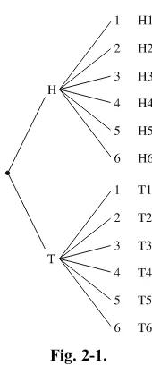
EXAMPLE: A coin is tossed and a die is rolled. Draw a tree diagram and find the sample space.
SOLUTION:
1. Since there are two outcomes (heads and tails for the coin), draw two branches from a single point and label one H for head and the other one T for tail.
2. From each one of these outcomes, draw and label six branches repre-senting the outcomes 1, 2, 3, 4, 5, and 6 for the die.
3. Trace through each branch to find the outcomes of the experiment. See Figure 2-1.
Hence there are twelve outcomes. They are H1, H2, H3, H4, H5, H6, T1, T2, T3, T4, T5, and T6.
Once the sample space has been found, probabilities for events can be computed.
Fig. 2-1.
EXAMPLE: A coin is tossed and a die is rolled. Find the probability of getting
a. A head on the coin and a 3 on the die. b. A head on the coin.
c. A 4 on the die.
SOLUTION:
a. Since there are 12 outcomes in the sample space and only one way to get a head on the coin and a three on the die,
PðH3Þ ¼ 1 12
b. Since there are six ways to get a head on the coin, namely H1, H2, H3, H4, H5, and H6,
Pðhead on the coin)¼ 6 12¼
1 2
c. Since there are two ways to get a 4 on the die, namely H4 and T4,
Pð4 on the die)¼ 2 12¼
1 6
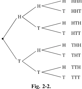
EXAMPLE:Three coins are tossed. Draw a tree diagram and find the sample space.
SOLUTION:
Each coin can land either heads up (H) or tails up (T); therefore, the tree diagram will consist of three parts and each part will have two branches. See Figure 2-2.
Fig. 2-2.
CHAPTER 2
Sample Spaces
Hence the sample space is HHH, HHT, HTH, HTT, THH, THT, TTH, TTT.
Once the sample space is found, probabilities can be computed.
EXAMPLE: Three coins are tossed. Find the probability of getting a. Two heads and a tail in any order.
b. Three heads. c. No heads.
d. At least two tails. e. At most two tails.
SOLUTION:
a. There are eight outcomes in the sample space, and there are three ways to get two heads and a tail in any order. They are HHT, HTH, and THH; hence,
P(2 heads and a tail)¼3 8
b. Three heads can occur in only one way; hence
PðHHHÞ ¼1 8
c. The event of getting no heads can occur in only one way—namely TTT; hence,
PðTTTÞ ¼1 8
d. The event of at least two tails means two tails and one head or three tails. There are four outcomes in this event—namely TTH, THT, HTT, and TTT; hence,
P(at least two tails)¼4 8¼
1 2
e. The event of getting at most two tails means zero tails, one tail, or two tails. There are seven outcomes in this event—HHH, THH, HTH, HHT, TTH, THT, and HTT; hence,
P(at most two tails)¼7 8
When selecting more than one object from a group of objects, it is important to know whether or not the object selected is replaced before drawing the second object. Consider the next two examples.
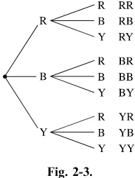
EXAMPLE:A box contains a red ball (R), a blue ball (B), and a yellow ball (Y). Two balls are selected at random in succession. Draw a tree diagram and find the sample space if the first ball is replaced before the second ball is selected.
SOLUTION:
There are three ways to select the first ball. They are a red ball, a blue ball, or a yellow ball. Since the first ball is replaced before the second one is selected, there are three ways to select the second ball. They are a red ball, a blue ball, or a yellow ball. The tree diagram is shown in Figure 2-3.
The sample space consists of nine outcomes. They are RR, RB, RY, BR, BB, BY, YR, YB, YY. Each outcome has a probability of 1
9:
Now what happens if the first ball is not replaced before the second ball is selected?
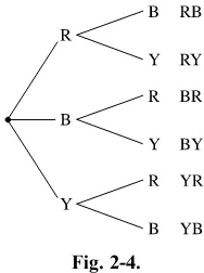
EXAMPLE:A box contains a red ball (R), a blue ball (B), and a yellow ball (Y). Two balls are selected at random in succession. Draw a tree diagram and find the sample space if the first ball is not replacedbefore the second ball is selected.
SOLUTION:
There are three outcomes for the first ball. They are a red ball, a blue ball, or a yellow ball. Since the first ball is not replaced before the second ball is drawn, there are only two outcomes for the second ball, and these outcomes depend on the color of the first ball selected. If the first ball selected is blue, then the second ball can be either red or yellow, etc. The tree diagram is shown in Figure 2-4.
Fig. 2-3.
CHAPTER 2
Sample Spaces
The sample space consists of six outcomes, which are RB, RY, BR, BY, YR, YB. Each outcome has a probability of 1
6:
PRACTICE
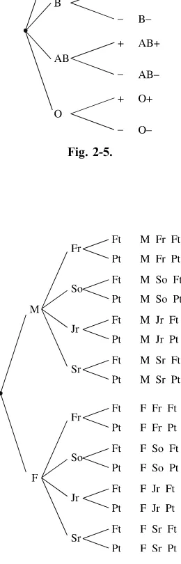
1. If the possible blood types are A, B, AB, and O, and each type can be Rhþ or Rh, draw a tree diagram and find all possible blood types. 2. Students are classified as male (M) or female (F), freshman (Fr), sophomore (So), junior (Jr), or senior (Sr), and full-time (Ft) or part-time (Pt). Draw a tree diagram and find all possible classifications. 3. A box contains a $1 bill, a $5 bill, and a $10 bill. Two bills are selected
in succession with replacement. Draw a tree diagram and find the sample space. Find the probability that the total amount of money selected is
a. $6.
b. Greater than $10. c. Less than $15.
4. Draw a tree diagram and find the sample space for the genders of the children in a family consisting of 3 children. Assume the genders are equiprobable. Find the probability of
a. Three girls.
b. Two boys and a girl in any order. c. At least two boys.
5. A box contains a white marble (W), a blue marble (B), and a green marble (G). Two marbles are selected without replacement. Draw a tree diagram and find the sample space. Find the probability that one marble is white.
Fig. 2-4.
ANSWERS
1.
2.
Fig. 2-6. Fig. 2-5.
CHAPTER 2
Sample Spaces
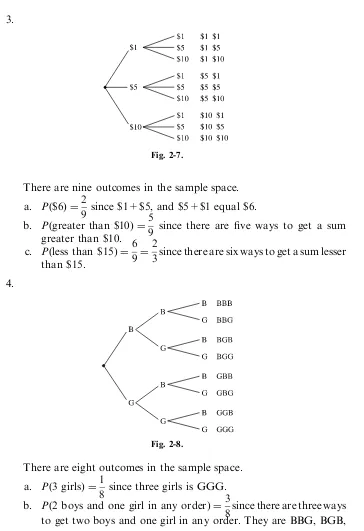
3.
There are nine outcomes in the sample space. a. Pð$6Þ ¼2
9 since $1+$5, and $5+$1 equal $6. b. Pðgreater than $10)¼5
9 since there are five ways to get a sum greater than $10.
c. Pðless than $15)¼6 9¼
2
3since there are six ways to get a sum lesser than $15.
4.
There are eight outcomes in the sample space. a. Pð3 girls)¼1
8 since three girls is GGG. b. P(2 boys and one girl in any order)¼3
8since there are three ways to get two boys and one girl in any order. They are BBG, BGB, and GBB.
Fig. 2-8. Fig. 2-7.
c. P(at least 2 boys)¼4 8¼
1
2 since at least two boys means two or three boys. The outcomes are BBG, BGB, GBB, and BBB. 5.
The probability that one marble is white is4 6¼
2
3since the outcomes are WB, WG, BW, and GW.
Tables
Another way to find a sample space is to use a table.
EXAMPLE:Find the sample space for selecting a card from a standard deck of 52 cards.
SOLUTION:
There are four suits—hearts and diamonds, which are red, and spades and clubs, which are black. Each suit consists of 13 cards—ace through king. Hence, the sample space can be shown using a table. See Figure 2-10.
Face cards are kings, queens, and jacks.
Once the sample space is found, probabilities for events can be computed.
Fig. 2-9.
Fig. 2-10.
CHAPTER 2
Sample Spaces
EXAMPLE: A single card is drawn at random from a standard deck of cards. Find the probability that it is
a. The 4 of diamonds. b. A queen.
c. A 5 or a heart.
SOLUTION:
a. The sample space consists of 52 outcomes and only one outcome is the four of diamonds; hence,
Pð4^Þ ¼ 1
52
b. Since there are four queens (one of each suit),
PðQÞ ¼ 4
52¼ 1 13
c. In this case, there are 13 hearts and 4 fives; however, the 5˘has been
counted twice, so the number of ways to get a 5 or a heart is 13þ41¼16. Hence,
Pð5 or˘Þ ¼16
52¼ 4 13:
A table can be used for the sample space when two dice are rolled. Since the first die can land in 6 ways and the second die can land in 6 ways, there are 66 or 36 outcomes in the sample space. It does not matter whether the two dice are of the same color or different color. The sample space is shown in Figure 2-11.
Fig. 2-11.
Notice that the sample space consists of ordered pairs of numbers. The outcome (4, 2) means that a 4 was obtained on the first die and a 2 was obtained on the second die. The sum of the spots on the faces in this case is 4þ2¼6. Probability problems involving rolling two dice can be solved using the sample space shown in Figure 2-11.
EXAMPLE: When two dice are rolled, find the probability of getting a sum of nine.
SOLUTION:
There are four ways of rolling a nine. They are (6, 3), (5, 4), (4, 5), and (3, 6). The sample space consists of 36 outcomes. Hence,
Pð9Þ ¼ 4 36¼
1 9
EXAMPLE: When two dice are rolled, find the probability of getting doubles.
SOLUTION:
There are six ways to get doubles. They are (1, 1), (2, 2), (3, 3), (4, 4), (5, 5), and (6, 6); hence
PðdoublesÞ ¼ 6 36¼
1 6
EXAMPLE: When two dice are rolled, find the probability of getting a sum less than five.
SOLUTION:
A sum less than five means a sum of four, three, or two. There are three ways of getting a sum of four. They are (3, 1), (2, 2), and (1, 3). There are two ways of getting a sum of three. They are (2, 1), and (1, 2). There is one way of getting a sum of two. It is (1, 1). The total number of ways of getting a sum less than five is 3þ2þ1¼6. Hence,
P(sum less than 6)¼ 6 36¼
1 6
CHAPTER 2
Sample Spaces
EXAMPLE: When two dice are rolled, find the probability that one of the numbers is a 6.
SOLUTION:
There are 11 outcomes that contain a 6. They are (1, 6), (2, 6), (3, 6), (4, 6), (5, 6), (6, 6), (6, 5), (6, 4), (6, 3), (6, 2), and (6, 1). Hence,
P(one of the numbers is a six)¼11 36
PRACTICE
1. When a card is selected at random, find the probability of getting a. A 9.
b. The ace of diamonds. c. A club.
2. When a card is selected at random from a deck, find the probability of getting
a. A black card. b. A red queen.
c. A heart or a spade.
3. When a card is selected at random from a deck, find the probability of getting
a. A diamond or a face card. b. A club or an 8.
c. A red card or a 6.
4. When two dice are rolled, find the probability of getting a. A sum of 7.
b. A sum greater than 8.
c. A sum less than or equal to 5.
5. When two dice are rolled, find the probability of getting a. A 5 on one or both dice.
b. A sum greater than 12. c. A sum less than 13.
ANSWERS
1. There are 52 outcomes in the sample space. a. There are four 9s, so
Pð9Þ ¼ 4 52¼
1 13
b. There is only one ace of diamonds, so
PðA^Þ ¼ 1
52
c. There are 13 clubs, so
Pð¨Þ ¼13
52¼ 1 4
2. There are 52 outcomes in the sample space.
a. There are 26 black cards: they are 13 clubs and 13 spades, so
Pðblack card)¼26 52¼
1 2
b. There are two red queens: they are the queen of diamonds and the queen of hearts, so
Pðred queen) = 2 52¼
1 26
c. There are 13 hearts and 13 spades, so
Pð˘ or ¨Þ ¼26
52¼ 1 2
3. There are 52 outcomes in the sample space.
a. There are 13 diamonds and 12 face cards, but the jack, queen, and king of diamonds have been counted twice, so
P(diamond or face card)¼13þ124 52 ¼
21 52
b. There are 13 clubs and four 8s, but the 8 of clubs has been counted twice, so
Pð¨ or an 8Þ ¼13þ41
52 ¼ 16 52¼
4 13
CHAPTER 2
Sample Spaces
c. There are 26 red cards and four 6s, but the 6 of hearts and the 6 of diamonds have been counted twice, so
Pðred card or 6)¼26þ42 52 ¼
28 52¼
7 13 4. There are 36 outcomes in the sample space.
a. There are six ways to get a sum of seven. They are (1, 6), (2, 5), (3, 4), (4, 3), (5, 2) and (6, 1); hence,
P(sum of 7)¼ 6 36¼
1 6
b. A sum greater than 8 means a sum of 9, 10, 11, 12, so
P(sum greater than 8)¼10 36¼
5 18
c. A sum less than or equal to five means a sum of five, four, three or two. There are ten ways to get a sum less than or equal to five; hence,
Pðsum less than or equal to fiveÞ ¼10 36¼
5 18 5. There are 36 outcomes in the sample space.
a. There are 11 ways to get a 5 on one or both dice. They are (1, 5), (2, 5), (3, 5), (4, 5), (5, 5), (6, 5), (5, 6), (5, 4), (5, 3) (5, 2), and (5, 1); hence,
P(5 on one or both dice)¼11 36
b. There are 0 ways to get a sum greater than 12; hence,
P(sum greater than 12)¼ 0 36¼0 The event is impossible.
c. Since all sums are less than 13 when two dice are rolled, there are 36 ways to get a sum less than 13; hence,
P(sum less than 13)¼36 36¼1 The event is certain.
Summary
Two devices can be used to represent sample spaces. They are tree diagrams and tables.
A tree diagram can be used to determine the outcome of a probability experiment. A tree diagram consists of branches corresponding to the outcomes of two or more probability experiments that are done in sequence. Sample spaces can also be represented by using tables. For example, the outcomes when selecting a card from an ordinary deck can be represented by a table. When two dice are rolled, the 36 outcomes can be represented by using a table. Once a sample space is found, probabilities can be computed for specific events.
CHAPTER QUIZ
1. When a coin is tossed and then a die is rolled, the probability of getting a tail on the coin and an odd number on the die is
a. 1 2 b. 1 4 c. 3 4 d. 1
12
2. When a coin is tossed and a die is rolled, the probability of getting a head and a number less than 5 on the die is
a. 1 3 b. 2 3 c. 1 2 d. 5 6
CHAPTER 2
Sample Spaces
3. When three coins are tossed, the probability of getting at least one tail is
a. 3 8 b. 1 8 c. 7 8 d. 5 8
4. When three coins are tossed, the probability of getting two or more heads is
a. 3 8 b. 1 8 c. 1 2 d. 7 8
5. A box contains a penny, a nickel, a dime, and a quarter. If two coins are selected without replacement, the probability of getting an amount greater than 11c is
a. 5 72 b. 2
3 c. 3 4 d. 5 6
6. A bag contains a red bead, a green bead, and a blue bead. If a bead is selected and its color noted, and then it is replaced and another bead is selected, the probability that both beads will be of the same color is
a. 1 8 b. 3 4 c. 1
16 d. 1
3
7. A card is selected at random from an ordinary deck of 52 cards. The probability that the 7 of diamonds is selected is
a. 1 13 b. 1
4 c. 1
52 d. 1
26
8. A card is selected at random from a deck of 52 cards. The probability that it is a 7 is
a. 1 4 b. 1
52 c. 7
52 d. 1
13
CHAPTER 2
Sample Spaces
9. A card is drawn from an ordinary deck of 52 cards. The probability that it is a spade is
a. 1 4 b. 1
13 c. 1
52 d. 1
26
10. A card is drawn from an ordinary deck of 52 cards. The probability that it is a 9 or a club is
a. 17 52 b. 5
8 c. 4
13 d. 3
4
11. A card is drawn from an ordinary deck of 52 cards. The probability that it is a face card is
a. 3 52 b. 1
4 c. 9
13 d. 3
13
12. Two dice are rolled. The probability that the sum of the spots on the faces will be nine is
a. 1 9 b. 5
36 c. 1
6 d. 3
13
13. Two dice are rolled. The probability that the sum of the spots on the faces is greater than seven is
a. 2 3 b. 7
36 c. 3
4 d. 5
12
14. Two dice are rolled. The probability that one or both numbers on the faces will be 4 is
a. 1 3 b. 4
13 c. 11 36 d. 1
6
CHAPTER 2
Sample Spaces
15. Two dice are rolled. The probability that the sum of the spots on the faces will be even is
a. 3 4 b. 5 6 c. 1 2 d. 1 6
Probability Sidelight
HISTORY OF DICE AND CARDS
Dice are one of the earliest known gambling devices used by humans. They have been found in ancient Egyptian tombs and in the prehistoric caves of people in Europe and America. The first dice were made from animal bones—namely the astragalus or the heel bone of a hoofed animal. These bones are very smooth and easily carved. The astragalus had only four sides as opposed to modern cubical dice that have six sides. The astragalus was used for fortune telling, gambling, and board games.
By 3000 B.C.E. the Egyptians had devised many board games. Ancient tomb paintings show pharaohs playing board games, and a game similar to today’s ‘‘Snakes and Ladders’’ was found in an Egyptian tomb dating to 1800 B.C.E. Eventually crude cubic dice evolved from the astragalus. The dice were first made from bones, then clay, wood, and finally polished stones. Dots were used instead of numbers since writing numbers was very complicated at that time.
It was thought that the outcomes of rolled dice were controlled by the gods that the people worshipped. As one story goes, the Romans incorrectly reasoned that there were three ways to get a sum of seven when two dice are rolled. They are 6 and 1, 5 and 2, and 4 and 3. They also reasoned incorrectly that there were three ways to get a sum of six: 5 and 1, 4 and 2, and 3 and 3.
They knew from gambling with dice that a sum of seven appeared more than a sum of six. They believed that the reason was that the gods favored the number seven over the number six, since seven at the time was considered a ‘‘lucky number.’’ Furthermore, they even ‘‘loaded’’ dice so that the faces showing one and six occurred more often than other faces would, if the dice were fair.
It is interesting to note that on today’s dice, the numbers on the opposite faces sum to seven. That is, 4 is opposite 3, 2 is opposite 5, and 6 is opposite 1. This was not always true. Early dice showed 1 opposite 2, 3 opposite 4, and 5 opposite 6. The changeover to modern configuration is believed to have occurred in Egypt.
Many of the crude dice have been tested and found to be quite accurate. Actually mathematicians began to study the outcomes of dice only around the 16th century. The great astronomer Galileo Galilei is usually given the credit for figuring out that when three dice are rolled, there are 216 total outcomes, and that a sum of 10 and 11 is more probable than a sum of 9 and 12. This fact was known intuitively by gamblers long before this time.
Today, dice are used in many types of gambling games and many types of board games. Where would we be today without the game of Monopoly?
It is thought that playing cards evolved from long wooden sticks that had various markings and were used by early fortunetellers and gamblers in the Far East. When the Chinese invented paper over 2000 years ago, people marked long thin strips of paper and used them instead of wooden sticks.
Paper ‘‘cards’’ first appeared in Europe around 1300 and were widely used in most of the European countries. Some decks contained 17 cards; others had 22 cards. The early cards were hand-painted and quite expensive to produce. Later stencils were used to cut costs.
The markings on the cards changed quite often. Besides the four suits commonly used today, early decks of cards had 5 or 6 suits and used other symbols such as coins, flowers, and leaves.
The first cards to be manufactured in the United States were made by Jazaniah Ford in the late 1700s. His company lasted over 50 years. The first book on gambling published in the United States was an edition of Hoyle’s Games, which was printed in 1796.
CHAPTER 2
Sample Spaces
CHAPTER
3
The Addition Rules
Introduction
In this chapter, the theory of probability is extended by using what are called the addition rules. Here one is interested in finding the probability of one event or another event occurring. In these situations, one must consider whether or not both events have common outcomes. For example, if you are asked to find the probability that you will get three oranges or three cherries on a slot machine, you know that these two events cannot occur at the same time if the machine has only three windows. In another situation you may be asked to find the probability of getting an odd number or a number less than 500 on a daily three-digit lottery drawing. Here the events have common outcomes. For example, the number 451 is an odd number and a number less than 500. The two addition rules will enable you to solve these kinds of problems as well as many other probability problems.
43
Mutually Exclusive Events
Many problems in probability involve finding the probability of two or more events. For example, when a card is selected at random from a deck, what is the probability that the card is a king or a queen? In this case, there are two situations to consider. They are:
1. The card selected is a king 2. The card selected is a queen
Now consider another example. When a card is selected from a deck, find the probability that the card is a king or a diamond.
In this case, there are three situations to consider: 1. The card is a king
2. The card is a diamond
3. The card is a king and a diamond. That is, the card is the king of diamonds.
The difference is that in the first example, a card cannot be both a king and a queen at the same time, whereas in the second example, it is possible for the card selected to be a king and a diamond at the same time. In the first example, we say the two events aremutually exclusive. In the second example, we say the two events are not mutually exclusive. Two events then are
mutually exclusiveif they cannot occur at the same time. In other words, the events have no common outcomes.
EXAMPLE: Which of these events are mutually exclusive?
a. Selecting a card at random from a deck and getting an ace or a club b. Rolling a die and getting an odd number or a number less than 4
c. Rolling two dice and getting a sum of 7 or 11
d. Selecting a student at random who is full-time or part-time e. Selecting a student who is a female or a junior
SOLUTION:
a. No. The ace of clubs is an outcome of both events. b. No. One and three are common outcomes.
c. Yes d. Yes
e. No. A female student who is a junior is a common outcome.
CHAPTER 3
The Addition Rules
Addition Rule I
The probability of two or more events occurring can be determined by using the addition rules. The first rule is used when the events are mutually exclusive.
Addition Rule I: When two events are mutually exclusive,
PðAor BÞ ¼PðAÞ þPðBÞ
EXAMPLE: When a die is rolled, find the probability of getting a 2 or a 3.
SOLUTION:
As shown in Chapter 1, the problem can be solved by looking at the sample space, which is 1, 2, 3, 4, 5, 6. Since there are 2 favorable outcomes from 6 outcomes, P(2 or 3)¼2
6¼13. Since the events are mutually exclusive,
addition rule 1 also can be used:
Pð2 or 3Þ ¼Pð2Þ þPð3Þ ¼1 6þ
1 6¼
2 6¼
1 3
EXAMPLE:In a committee meeting, there were 5 freshmen, 6 sophomores, 3 juniors, and 2 seniors. If a student is selected at random to be the chairperson, find the probability that the chairperson is a sophomore or a junior.
SOLUTION:
There are 6 sophomores and 3 juniors and a total of 16 students.
P(sophomore or junior)¼PðsophomoreÞ þPðjuniorÞ ¼ 6 16þ
3 16¼
9 16
EXAMPLE:A card is selected at random from a deck. Find the probability that the card is an ace or a king.
SOLUTION:
P(ace or king)¼PðaceÞ þPðkingÞ ¼ 4 52þ
4 52¼
8 52¼
2 13
The word oris the key word, and it means one event occurs or the other event occurs.
PRACTICE
1. In a box there are 3 red pens, 5 blue pens, and 2 black pens. If a person selects a pen at random, find the probability that the pen is
a. A blue or a red pen. b. A red or a black pen.
2. A small automobile dealer has 4 Buicks, 7 Fords, 3 Chryslers, and 6 Chevrolets. If a car is selected at random, find the probability that it is
a. A Buick or a Chevrolet. b. A Chrysler or a Chevrolet.
3. In a model railroader club, 23 members model HO scale, 15 members model N scale, 10 members model G scale, and 5 members model O scale. If a member is selected at random, find the probability that the member models
a. N or G scale. b. HO or O scale.
4. A package of candy contains 8 red pieces, 6 white pieces, 2 blue pieces, and 4 green pieces. If a piece is selected at random, find the probability that it is
a. White or green. b. Blue or red.
5. On a bookshelf in a classroom there are 6 mathematics books, 5 reading books, 4 science books, and 10 history books. If a student selects a book at random, find the probability that the book is
a. A history book or a mathematics book. b. A reading book or a science book.
ANSWERS
1. a. P(blue or red)¼P(blue)þP(red)¼ 5 10þ
3 10¼
8 10¼
4 5
b. P(red or black)¼P(red)þP(black)¼ 3 10þ
2 10¼
5 10¼
1 2
CHAPTER 3
The Addition Rules
2. a. P(Buick or Chevrolet)¼P(Buick)þP(Chevrolet)
¼204 þ206 ¼1020¼12
b. P(Chrysler or Chevrolet)¼P(Chrysler)þP(Chevrolet)
¼203 þ206 ¼209
3. a. P(N or G)¼P(N)þP(G)¼15 53þ
10 53¼
25 53
b. P(HO or O)¼P(HO)þP(O)¼23 53þ
5 53¼
28 53
4. a. P(white or green)¼P(white)þP(green)¼ 6 20þ 4 20¼ 10 20¼ 1 2
b. P(blue or red)¼P(blue)þP(red)¼ 2 20þ 8 20¼ 10 20¼ 1 2
5. a. P(history or math)¼P(history)þP(math)¼10 25þ
6 25¼
16 25
b. P(reading or science)¼P(reading)þP(science)¼ 5 25þ
4 25¼
9 25
Addition Rule II
When two events are not mutually exclusive, you need to add the probabilities of each of the two events and subtract the probability of the outcomes that are common to both events. In this case, addition rule II can be used.
Addition Rule II: IfAand Bare two events that are not mutually exclusive, thenPðAor BÞ ¼PðAÞ þPðBÞ PðAand BÞ, whereAandBmeans the num-ber of outcomes that eventAand eventBhave in common.
EXAMPLE:A card is selected at random from a deck of 52 cards. Find the probability that it is a 6 or a diamond.
SOLUTION:
Let A¼the event of getting a 6; then PðAÞ ¼ 4
52 since there are four 6s.
Let B¼the event of getting a diamond; then PðBÞ ¼1352 since there are 13 diamonds. Since there is one card that is both a 6 and a diamond (i.e., the 6 of diamonds), PðAand BÞ ¼ 1
52. Hence,
PðAor BÞ ¼PðAÞ þPðBÞ PðAand BÞ ¼ 4
52þ 13 52 1 52¼ 16 52¼ 4 13
EXAMPLE: A die is rolled. Find the probability of getting an even number or a number less than 4.
SOLUTION:
LetA¼an even number; thenPðAÞ ¼3
6since there are 3 even numbers—2, 4,
and 6. LetB¼a number less than 4; thenPðBÞ ¼36since there are 3 numbers less than 4—1, 2, and 3. Let (A and B)¼even numbers less than 4 and
PðAand BÞ ¼16since there is one even number less than 4—namely 2. Hence,
PðAor BÞ ¼PðAÞ þPðBÞ PðAand BÞ ¼3
6þ 3 6 1 6¼ 5 6
The results of both these examples can be verified by using sample spaces and classical probability.
EXAMPLE:Two dice are rolled; find the probability of getting doubles or a sum of 8.
SOLUTION:
LetA¼getting doubles; thenPðAÞ ¼366 since there are 6 ways to get doubles and letB¼getting a sum of 8. ThenPðBÞ ¼ 5
36since there are 5 ways to get a
sum of 8—(6, 2), (5, 3), (4, 4), (3, 5), and (2, 6). Let (AandB)¼the number of ways to get a double and a sum of 8. There is only one way for this event