MITgcm User Manual
Alistair Adcroft
Jean-Michel Campin
Stephanie Dutkiewicz
Constantinos Evangelinos
David Ferreira
Gael Forget
Baylor Fox-Kemper
Patrick Heimbach
Chris Hill
Ed Hill
Helen Hill
Oliver Jahn
Martin Losch
John Marshall
Guillaume Maze
Dimitris Menemenlis
Andrea Molod
MIT Department of EAPS
77 Massachusetts Ave.
Cambridge, MA 02139-4307
Contents
1 Overview of MITgcm 9
1.1 Introduction. . . 9
1.2 Illustrations of the model in action . . . 13
1.2.1 Global atmosphere: ‘Held-Suarez’ benchmark . . . 13
1.2.2 Ocean gyres. . . 14
1.2.3 Global ocean circulation . . . 14
1.2.4 Convection and mixing over topography . . . 14
1.2.5 Boundary forced internal waves . . . 14
1.2.6 Parameter sensitivity using the adjoint of MITgcm . . . 14
1.2.7 Global state estimation of the ocean . . . 20
1.2.8 Ocean biogeochemical cycles . . . 20
1.2.9 Simulations of laboratory experiments . . . 20
1.3 Continuous equations in ‘r’ coordinates. . . 23
1.3.1 Kinematic Boundary conditions. . . 26
1.3.2 Atmosphere . . . 26
1.3.3 Ocean . . . 27
1.3.4 Hydrostatic, Quasi-hydrostatic, Quasi-nonhydrostatic and Non-hydrostatic forms . 27 1.3.5 Solution strategy . . . 30
1.3.6 Finding the pressure field . . . 31
1.3.7 Forcing/dissipation . . . 33
1.3.8 Vector invariant form . . . 33
1.3.9 Adjoint . . . 33
1.4 Appendix ATMOSPHERE. . . 34
1.4.1 Hydrostatic Primitive Equations for the Atmosphere in pressure coordinates. . . . 34
1.5 Appendix OCEAN . . . 36
1.5.1 Equations of motion for the ocean . . . 36
1.6 Appendix:OPERATORS . . . 39
1.6.1 Coordinate systems . . . 39
2 Discretization and Algorithm 41 2.1 Notation . . . 41
2.2 Time-stepping. . . 41
2.3 Pressure method with rigid-lid . . . 42
2.4 Pressure method with implicit linear free-surface . . . 44
2.5 Explicit time-stepping: Adams-Bashforth . . . 44
2.6 Implicit time-stepping: backward method . . . 45
2.7 Synchronous time-stepping: variables co-located in time . . . 47
2.8 Staggered baroclinic time-stepping . . . 49
2.9 Non-hydrostatic formulation. . . 51
2.10 Variants on the Free Surface. . . 53
2.10.1 Crank-Nicolson barotropic time stepping. . . 54
2.10.2 Non-linear free-surface . . . 55
2.11 Spatial discretization of the dynamical equations . . . 59
2.11.1 The finite volume method: finite volumes versus finite difference . . . 59 3
2.11.2 C grid staggering of variables . . . 60
2.11.3 Grid initialization and data . . . 60
2.11.4 Horizontal grid . . . 61
2.11.5 Vertical grid . . . 63
2.11.6 Topography: partially filled cells . . . 64
2.12 Continuity and horizontal pressure gradient terms . . . 65
2.13 Hydrostatic balance . . . 65
2.14 Flux-form momentum equations . . . 66
2.14.1 Advection of momentum. . . 66
2.14.2 Coriolis terms. . . 67
2.14.3 Curvature metric terms . . . 67
2.14.4 Non-hydrostatic metric terms . . . 68
2.14.5 Lateral dissipation . . . 68
2.14.6 Vertical dissipation. . . 69
2.14.7 Derivation of discrete energy conservation . . . 70
2.14.8 Mom Diagnostics . . . 70
2.15 Vector invariant momentum equations . . . 72
2.15.1 Relative vorticity . . . 72
2.15.2 Kinetic energy . . . 72
2.15.3 Coriolis terms. . . 73
2.15.4 Shear terms . . . 73
2.15.5 Gradient of Bernoulli function . . . 73
2.15.6 Horizontal divergence . . . 74
2.15.7 Horizontal dissipation . . . 74
2.15.8 Vertical dissipation. . . 74
2.16 Tracer equations . . . 75
2.16.1 Time-stepping of tracers: ABII . . . 75
2.17 Linear advection schemes . . . 76
2.17.1 Centered second order advection-diffusion . . . 78
2.17.2 Third order upwind bias advection . . . 78
2.17.3 Centered fourth order advection . . . 79
2.17.4 First order upwind advection . . . 79
2.18 Non-linear advection schemes . . . 80
2.18.1 Second order flux limiters . . . 80
2.18.2 Third order direct space time . . . 80
2.18.3 Third order direct space time with flux limiting. . . 81
2.18.4 Multi-dimensional advection. . . 85
2.19 Comparison of advection schemes . . . 85
2.20 Shapiro Filter . . . 87
2.20.1 SHAP Diagnostics . . . 88
2.21 Nonlinear Viscosities for Large Eddy Simulation . . . 88
2.21.1 Eddy Viscosity . . . 89
2.21.2 Mercator, Nondimensional Equations. . . 92
3 Getting Started with MITgcm 95 3.1 Where to find information . . . 95
3.2 Obtaining the code . . . 95
3.2.1 Method 1 - Checkout from CVS . . . 95
3.2.2 Method 2 - Tar file download . . . 97
3.3 Model and directory structure . . . 98
3.4 Building MITgcm. . . 98
3.4.1 Building/compiling the code elsewhere . . . 99
3.4.2 Usinggenmake2 . . . 101
3.4.3 Building with MPI . . . 103
3.5 Running MITgcm. . . 104
CONTENTS 5
3.5.2 Looking at the output . . . 105
3.6 Customizing MITgcm . . . 107
3.6.1 Parameters: Computational domain, geometry and time-discretization . . . 108
3.6.2 Parameters: Equation of state . . . 113
3.6.3 Parameters: Momentum equations . . . 114
3.6.4 Parameters: Tracer equations . . . 115
3.6.5 Parameters: Simulation controls . . . 116
3.7 Testing . . . 117
3.7.1 Usingtestreport . . . 117
3.7.2 Automated testing . . . 117
3.8 MITgcm Example Experiments . . . 118
3.8.1 Full list of model examples . . . 118
3.8.2 Directory structure of model examples . . . 122
3.9 Barotropic Gyre MITgcm Example . . . 124
3.9.1 Equations Solved . . . 124
3.9.2 Discrete Numerical Configuration. . . 124
3.9.3 Code Configuration . . . 126
3.10 Baroclinic Gyre MITgcm Example . . . 131
3.10.1 Overview . . . 131
3.10.2 Equations solved . . . 131
3.10.3 Discrete Numerical Configuration. . . 133
3.10.4 Code Configuration . . . 135
3.10.5 Running The Example . . . 140
3.11 Gyre Advection Example . . . 141
3.11.1 Advection and tracer transport . . . 141
3.11.2 Introducing a tracer into the flow . . . 141
3.11.3 Selecting an advection scheme. . . 142
3.11.4 Comparison of different advection schemes. . . 142
3.11.5 Code and Parameters files for this tutorial . . . 142
3.12 Global Ocean MITgcm Example . . . 143
3.12.1 Overview . . . 143
3.12.2 Discrete Numerical Configuration. . . 144
3.12.3 Experiment Configuration . . . 145
3.13 P coordinate Global Ocean MITgcm Example . . . 153
3.13.1 Overview . . . 153
3.13.2 Discrete Numerical Configuration. . . 153
3.13.3 Experiment Configuration . . . 155
3.14 Held-Suarez Atmosphere MITgcm Example . . . 169
3.14.1 Overview . . . 169
3.14.2 Forcing . . . 169
3.14.3 Set-up description . . . 170
3.14.4 Experiment Configuration . . . 171
3.15 Surface Driven Convection. . . 180
3.15.1 Overview . . . 180
3.15.2 Equations solved . . . 182
3.15.3 Discrete numerical configuration . . . 182
3.15.4 Numerical stability criteria and other considerations . . . 182
3.15.5 Experiment configuration . . . 183
3.15.6 Running the example . . . 190
3.16 Gravity Plume On a Continental Slope. . . 191
3.16.1 Configuration . . . 192
3.16.2 Binary input data . . . 192
3.16.3 Code configuration . . . 194
3.16.4 Model parameters . . . 195
3.16.5 Build and run the model. . . 195
3.17.1 Overview . . . 196
3.17.2 Equations Solved . . . 197
3.17.3 Code configuration . . . 197
3.17.4 Running the example . . . 199
3.18 Global Ocean State Estimation Example . . . 200
3.18.1 Overview . . . 200
3.18.2 Implementation of the control variable and the cost function . . . 201
3.18.3 Code Configuration . . . 202
3.18.4 Compiling . . . 203
3.18.5 Running the estimation . . . 204
3.19 Sensitivity of Air-Sea Exchange to Tracer Injection Site . . . 205
3.19.1 Overview of the experiment . . . 205
3.19.2 Code configuration . . . 205
3.19.3 Compiling the model and its adjoint . . . 210
3.20 Offline Example. . . 212
3.20.1 Overview . . . 212
3.20.2 Time-stepping of tracers . . . 212
3.20.3 Code Configuration . . . 212
3.20.4 Running The Example . . . 219
3.20.5 A more complicated example . . . 220
3.21 A Rotating Tank in Cylindrical Coordinates . . . 225
3.21.1 Overview . . . 225
3.21.2 Equations Solved . . . 225
3.21.3 Discrete Numerical Configuration. . . 225
3.21.4 Code Configuration . . . 225
4 Software Architecture 231 4.1 Overall architectural goals . . . 231
4.2 WRAPPER . . . 232
4.2.1 Target hardware . . . 232
4.2.2 Supporting hardware neutrality . . . 232
4.2.3 WRAPPER machine model . . . 234
4.2.4 Machine model parallelism . . . 234
4.2.5 Communication mechanisms . . . 234
4.2.6 Shared memory communication . . . 236
4.2.7 Distributed memory communication . . . 237
4.2.8 Communication primitives. . . 238
4.2.9 Memory architecture . . . 239
4.2.10 Summary . . . 240
4.3 Using the WRAPPER . . . 240
4.3.1 Specifying a domain decomposition. . . 240
4.3.2 Starting the code . . . 245
4.3.3 Controlling communication . . . 248
4.4 MITgcm execution under WRAPPER . . . 252
4.4.1 Annotated call tree for MITgcm and WRAPPER. . . 252
4.4.2 Measuring and Characterizing Performance . . . 257
4.4.3 Estimating Resource Requirements . . . 257
5 Automatic Differentiation 259 5.1 Some basic algebra . . . 259
5.1.1 Forward or direct sensitivity. . . 260
5.1.2 Reverse or adjoint sensitivity . . . 260
5.1.3 Storing vs. recomputation in reverse mode . . . 263
5.2 TLM and ADM generation in general . . . 264
5.2.1 General setup . . . 264
CONTENTS 7
5.2.3 The AD build process in detail . . . 266
5.2.4 The cost function (dependent variable) . . . 268
5.2.5 The control variables (independent variables) . . . 269
5.3 The gradient check package . . . 275
5.3.1 Code description . . . 275
5.3.2 Code configuration . . . 275
5.4 Adjoint dump & restart – divided adjoint (DIVA) . . . 276
5.4.1 Introduction . . . 276
5.4.2 Recipe 1: single processor . . . 277
5.4.3 Recipe 2: multi processor (MPI) . . . 278
5.5 Adjoint code generation using OpenAD . . . 279
5.5.1 Introduction . . . 279
5.5.2 Downloading and installing OpenAD . . . 279
5.5.3 Building MITgcm adjoint with OpenAD . . . 279
6 Physical Parameterizations - Packages I 281 6.1 Using MITgcm Packages . . . 283
6.1.1 Package Inclusion/Exclusion . . . 283
6.1.2 Package Activation . . . 283
6.1.3 Package Coding Standards . . . 283
6.2 Packages Related to Hydrodynamical Kernel . . . 287
6.2.1 Generic Advection/Diffusion . . . 287
6.2.2 Shapiro Filter . . . 288
6.2.3 FFT Filtering Code . . . 289
6.2.4 exch2: Extended Cubed Sphere Topology . . . 290
6.2.5 Gridalt - Alternate Grid Package . . . 297
6.3 General purpose numerical infrastructure packages . . . 301
6.3.1 OBCS: Open boundary conditions for regional modeling . . . 301
6.3.2 RBCS Package . . . 307
6.3.3 PTRACERS Package . . . 309
6.4 Ocean Packages . . . 312
6.4.1 GMREDI: Gent-McWilliams/Redi SGS Eddy Parameterization . . . 312
6.4.2 KPP: Nonlocal K-Profile Parameterization for Vertical Mixing . . . 318
6.4.3 GGL90: a TKE vertical mixing scheme . . . 323
6.4.4 OPPS: Ocean Penetrative Plume Scheme . . . 324
6.4.5 KL10: Vertical Mixing Due to Breaking Internal Waves . . . 325
6.4.6 BULK FORCE: Bulk Formula Package . . . 328
6.4.7 EXF: The external forcing package . . . 332
6.4.8 CAL: The calendar package . . . 338
6.5 Atmosphere Packages . . . 342
6.5.1 Atmospheric Intermediate Physics: AIM . . . 342
6.5.2 Land package . . . 343
6.5.3 Fizhi: High-end Atmospheric Physics. . . 345
6.6 Sea Ice Packages . . . 380
6.6.1 THSICE: The Thermodynamic Sea Ice Package . . . 380
6.6.2 SEAICE Package . . . 385
6.6.3 SHELFICE Package . . . 397
6.6.4 STREAMICE Package . . . 402
6.7 Packages Related to Coupled Model . . . 408
6.7.1 Coupling interface for Atmospheric Intermediate code . . . 408
6.7.2 Coupler for mapping between Atmosphere and ocean . . . 409
6.7.3 Toolkit for building couplers . . . 410
6.8 Biogeochemistry Packages . . . 411
6.8.1 GCHEM Package. . . 411
7 Diagnostics and I/O - Packages II, and Post–Processing Utilities 417
7.1 Diagnostics–A Flexible Infrastructure . . . 417
7.1.1 Introduction . . . 417
7.1.2 Equations . . . 417
7.1.3 Key Subroutines and Parameters . . . 417
7.1.4 Usage Notes. . . 421
7.1.5 Dos and Donts . . . 428
7.1.6 Diagnostics Reference . . . 428
7.2 NetCDF I/O: MNC . . . 429
7.2.1 Using MNC . . . 429
7.2.2 MNC Troubleshooting . . . 432
7.2.3 MNC Internals . . . 432
7.3 Fortran Native I/O: MDSIO and RW. . . 435
7.3.1 MDSIO . . . 435
7.3.2 RW Basic binary I/O utilities . . . 437
7.4 Monitor: Simulation state monitoring toolkit . . . 438
7.4.1 Introduction . . . 438
7.4.2 Using Monitor . . . 438
7.5 Grid Generation . . . 439
7.5.1 Using SPGrid. . . 439
7.5.2 Example Grids . . . 440
7.6 Pre– and Post–Processing Scripts and Utilities . . . 441
7.6.1 Utilities supplied with the model . . . 441
7.6.2 Pre-processing software . . . 441
7.7 Potential vorticity Matlab Toolbox . . . 442
7.7.1 Introduction . . . 442
7.7.2 Equations . . . 442
7.7.3 Key routines . . . 443
7.7.4 Technical details . . . 444
7.7.5 Notes on the flux form of the PV equation and vertical PV fluxes. . . 445
8 Ocean State Estimation Packages 449 8.1 ECCO: model-data comparisons using gridded data sets . . . 449
8.1.1 Generic Cost Function . . . 449
8.1.2 Generic Integral Function . . . 453
8.1.3 Custom Cost Functions . . . 453
8.1.4 Key Routines . . . 453
8.1.5 Compile Options . . . 453
8.2 PROFILES: model-data comparisons at observed locations . . . 454
8.3 CTRL: Model Parameter Adjustment Capability . . . 457
8.4 SMOOTH: Smoothing And Covariance Model . . . 459
8.5 The line search optimisation algorithm . . . 460
8.5.1 General features . . . 460
8.5.2 The online vs. offline version . . . 460
8.5.3 Number of iterations vs. number of simulations . . . 460
9 Under development 465 9.1 Other Time-stepping Options . . . 465
9.1.1 Adams-Bashforth III . . . 465
9.1.2 Time-extrapolation of tracer (rather than tendency) . . . 467
10 Previous Applications of MITgcm 469
Chapter 1
Overview of MITgcm
This document provides the reader with the information necessary to carry out numerical experiments using MITgcm. It gives a comprehensive description of the continuous equations on which the model is based, the numerical algorithms the model employs and a description of the associated program code. Along with the hydrodynamical kernel, physical and biogeochemical parameterizations of key atmospheric and oceanic processes are available. A number of examples illustrating the use of the model in both process and general circulation studies of the atmosphere and ocean are also presented.
1.1
Introduction
MITgcm has a number of novel aspects:
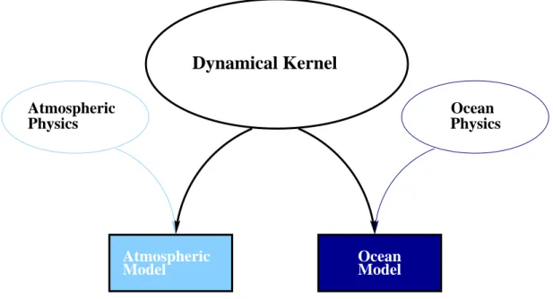
• it can be used to study both atmospheric and oceanic phenomena; one hydrodynamical kernel is used to drive forward both atmospheric and oceanic models - see fig1.1
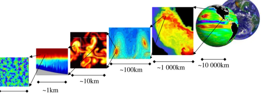
• it has a non-hydrostatic capability and so can be used to study both small-scale and large scale processes - see fig1.2
• finite volume techniques are employed yielding an intuitive discretization and support for the treat-ment of irregular geometries using orthogonal curvilinear grids and shaved cells - see fig1.3
• tangent linear and adjoint counterparts are automatically maintained along with the forward model, permitting sensitivity and optimization studies.
• the model is developed to perform efficiently on a wide variety of computational platforms. Key publications reporting on and charting the development of the model are Hill and Marshall [1995];Marshall et al.[1997b,a];Adcroft et al.[1997];Marshall et al.[1998];Adcroft and Marshall[1999]; Chris Hill and Marshall[1999];Marotzke et al.[1999];Adcroft and Campin [2004];Adcroft et al.[2004a]; Marshall et al.[2004] (an overview on the model formulation can also be found inAdcroft et al.[2004b]):
Hill, C. and J. Marshall, (1995)
Application of a Parallel Navier-Stokes Model to Ocean Circulation in Parallel Computational Fluid Dynamics
In Proceedings of Parallel Computational Fluid Dynamics: Implementations and Results Using Parallel Computers, 545-552.
Elsevier Science B.V.: New York
Marshall, J., C. Hill, L. Perelman, and A. Adcroft, (1997)
Hydrostatic, quasi-hydrostatic, and nonhydrostatic ocean modeling J. Geophysical Res., 102(C3), 5733-5752.
Marshall, J., A. Adcroft, C. Hill, L. Perelman, and C. Heisey, (1997)
A finite-volume, incompressible Navier Stokes model for studies of the ocean
Atmospheric
Ocean
Dynamical Kernel
Atmospheric
Physics
Model
Model
Ocean
Physics
Figure 1.1: MITgcm has a single dynamical kernel that can drive forward either oceanic or atmospheric simulations.
on parallel computers,
J. Geophysical Res., 102(C3), 5753-5766.
Adcroft, A.J., Hill, C.N. and J. Marshall, (1997)
Representation of topography by shaved cells in a height coordinate ocean model
Mon Wea Rev, vol 125, 2293-2315
Marshall, J., Jones, H. and C. Hill, (1998)
Efficient ocean modeling using non-hydrostatic algorithms Journal of Marine Systems, 18, 115-134
Adcroft, A., Hill C. and J. Marshall: (1999)
A new treatment of the Coriolis terms in C-grid models at both high and low resolutions,
Mon. Wea. Rev. Vol 127, pages 1928-1936
Hill, C, Adcroft,A., Jamous,D., and J. Marshall, (1999) A Strategy for Terascale Climate Modeling.
In Proceedings of the Eighth ECMWF Workshop on the Use of Parallel Processors in Meteorology, pages 406-425
World Scientific Publishing Co: UK
Marotzke, J, Giering,R., Zhang, K.Q., Stammer,D., Hill,C., and T.Lee, (1999) Construction of the adjoint MIT ocean general circulation model and
application to Atlantic heat transport variability J. Geophysical Res., 104(C12), 29,529-29,547.
We begin by briefly showing some of the results of the model in action to give a feel for the wide range of problems that can be addressed using it.
1.1. INTRODUCTION 11 ~10 000km ~1 000km ~100km ~1km ~10km ~100m
Figure 1.2: MITgcm has non-hydrostatic capabilities, allowing the model to address a wide range of phenomenon - from convection on the left, all the way through to global circulation patterns on the right.
nite Volume: Shaved cells
Figure 1.3: Finite volume techniques (bottom panel) are user, permitting a treatment of topography that rivalsσ(terrain following) coordinates.
1.2. ILLUSTRATIONS OF THE MODEL IN ACTION 13
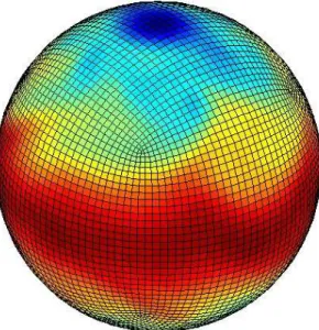
Figure 1.4: Instantaneous plot of the temerature field at 500mb obtained using the atmospheric isomorph of MITgcm
1.2
Illustrations of the model in action
MITgcm has been designed and used to model a wide range of phenomena, from convection on the scale of meters in the ocean to the global pattern of atmospheric winds - see figure 1.2. To give a flavor of the kinds of problems the model has been used to study, we briefly describe some of them here. A more detailed description of the underlying formulation, numerical algorithm and implementation that lie behind these calculations is given later. Indeed many of the illustrative examples shown below can be easily reproduced: simply download the model (the minimum you need is a PC running Linux, together with a FORTRAN 77 compiler) and follow the examples described in detail in the documentation.
1.2.1
Global atmosphere: ‘Held-Suarez’ benchmark
A novel feature of MITgcm is its ability to simulate, using one basic algorithm, both atmospheric and oceanographic flows at both small and large scales.
Figure1.4shows an instantaneous plot of the 500mbtemperature field obtained using the atmospheric isomorph of MITgcm run at 2.8◦ resolution on the cubed sphere. We see cold air over the pole (blue)
and warm air along an equatorial band (red). Fully developed baroclinic eddies spawned in the northern hemisphere storm track are evident. There are no mountains or land-sea contrast in this calculation, but you can easily put them in. The model is driven by relaxation to a radiative-convective equilibrium profile, following the description set out in Held and Suarez; 1994 designed to test atmospheric hydrodynamical cores - there are no mountains or land-sea contrast.
As described in Adcroft (2001), a ‘cubed sphere’ is used to discretize the globe permitting a uniform griding and obviated the need to Fourier filter. The ‘vector-invariant’ form of MITgcm supports any orthogonal curvilinear grid, of which the cubed sphere is just one of many choices.
Figure 1.5 shows the 5-year mean, zonally averaged zonal wind from a 20-level configuration of the model. It compares favorable with more conventional spatial discretization approaches. The two plots show the field calculated using the cube-sphere grid and the flow calculated using a regular, spherical polar latitude-longitude grid. Both grids are supported within the model.
1.2.2
Ocean gyres
Baroclinic instability is a ubiquitous process in the ocean, as well as the atmosphere. Ocean eddies play an important role in modifying the hydrographic structure and current systems of the oceans. Coarse resolution models of the oceans cannot resolve the eddy field and yield rather broad, diffusive patterns of ocean currents. But if the resolution of our models is increased until the baroclinic instability process is resolved, numerical solutions of a different and much more realistic kind, can be obtained.
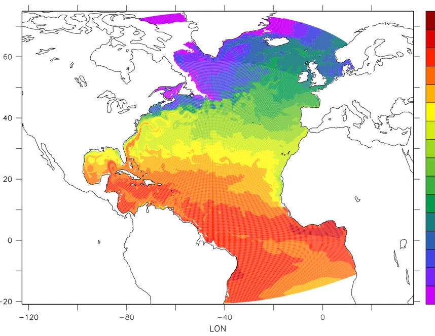
Figure1.6shows the surface temperature and velocity field obtained from MITgcm run at16◦horizontal resolution on a lat-lon grid in which the pole has been rotated by 90◦ on to the equator (to avoid the
converging of meridian in northern latitudes). 21 vertical levels are used in the vertical with a ‘lopped cell’ representation of topography. The development and propagation of anomalously warm and cold eddies can be clearly seen in the Gulf Stream region. The transport of warm water northward by the mean flow of the Gulf Stream is also clearly visible.
1.2.3
Global ocean circulation
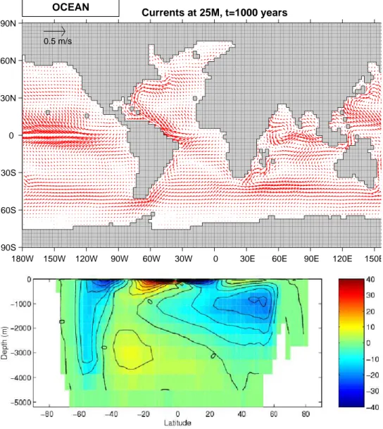
Figure1.7(top) shows the pattern of ocean currents at the surface of a 4◦ global ocean model run with
15 vertical levels. Lopped cells are used to represent topography on a regular lat-lon grid extending from 70◦N to 70◦S. The model is driven using monthly-mean winds with mixed boundary conditions on
temperature and salinity at the surface. The transfer properties of ocean eddies, convection and mixing is parameterized in this model.
Figure 1.7(bottom) shows the meridional overturning circulation of the global ocean in Sverdrups.
1.2.4
Convection and mixing over topography
Dense plumes generated by localized cooling on the continental shelf of the ocean may be influenced by rotation when the deformation radius is smaller than the width of the cooling region. Rather than gravity plumes, the mechanism for moving dense fluid down the shelf is then through geostrophic eddies. The simulation shown in the figure1.8(blue is cold dense fluid, red is warmer, lighter fluid) employs the non-hydrostatic capability of MITgcm to trigger convection by surface cooling. The cold, dense water falls down the slope but is deflected along the slope by rotation. It is found that entrainment in the vertical plane is reduced when rotational control is strong, and replaced by lateral entrainment due to the baroclinic instability of the along-slope current.
1.2.5
Boundary forced internal waves
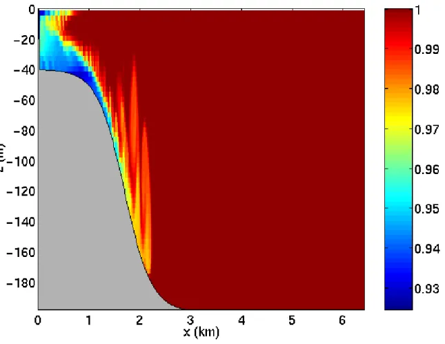
The unique ability of MITgcm to treat non-hydrostatic dynamics in the presence of complex geometry makes it an ideal tool to study internal wave dynamics and mixing in oceanic canyons and ridges driven by large amplitude barotropic tidal currents imposed through open boundary conditions.
Fig. 1.9 shows the influence of cross-slope topographic variations on internal wave breaking - the cross-slope velocity is in color, the density contoured. The internal waves are excited by application of open boundary conditions on the left. They propagate to the sloping boundary (represented using MITgcm’s finite volume spatial discretization) where they break under nonhydrostatic dynamics.
1.2.6
Parameter sensitivity using the adjoint of MITgcm
Forward and tangent linear counterparts of MITgcm are supported using an ‘automatic adjoint compiler’. These can be used in parameter sensitivity and data assimilation studies.
As one example of application of the MITgcm adjoint, Figure1.10maps the gradient ∂∂JHwhereJ is the magnitude of the overturning stream-function shown in figure1.7at 60◦N andH(λ, ϕ) is the mean,
1.2. ILLUSTRATIONS OF THE MODEL IN ACTION 15
Figure 1.5: Five year mean, zonally averaged zonal flow for latitude-longitude simulation (bottom) and cube-sphere simulation(top) using Held-Suarez forcing. Note the difference in the solutions over the pole - the cubed sphere is superior.
Figure 1.6: Instantaneous temperature map from a 16◦simulation of the North Atlantic. The figure shows the temperature in the second layer (37.5m deep).
1.2. ILLUSTRATIONS OF THE MODEL IN ACTION 17
180W 150W 120W 90W 60W 30W 0 30E 60E 90E 120E 150E 90S 60S 30S 0 30N 60N 90N Currents at 25M, t=1000 years 0.5 m/s OCEAN
Figure 1.7: Pattern of surface ocean currents (top) and meridional overturning stream function (in Sverdrups) from a global integration of the model at 4◦horizontal resolution and with 15 vertical levels.
1.2. ILLUSTRATIONS OF THE MODEL IN ACTION 19
Figure 1.9: Simulation of internal waves forced at an open boundary (on the left) impacting a sloping shelf. The along slope velocity is shown colored, contour lines show density surfaces. The slope is represented with high-fidelity using lopped cells.
180W 150W 120W 90W 60W 30W 0 30E 60E 90E 120E 150E 180E 90S 60S 30S 0 30N 60N 90N
Heat Flux (Min = −7.7 10−4 Sv W−1 m2; Max = 42.9 10−4 Sv W−1 m2)
−10 −5 0 5 10 15 20 25 30 35 40 45 50
10−4 Sv W−1 m2
Figure 1.10: Sensitivity of meridional overturning strength to surface heat flux changes. Contours show the magnitude of the response (in Sv×10−4) that a persistent +1Wm−2 heat flux anomaly at a given
gid point would produce.
Sea, one of the important sources of deep water for the thermohaline circulations. This calculation also yields sensitivities to all other model parameters.
1.2.7
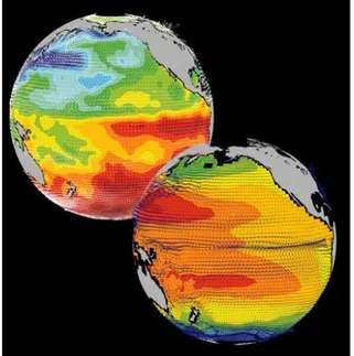
Global state estimation of the ocean
An important application of MITgcm is in state estimation of the global ocean circulation. An appropri-ately defined ‘cost function’, which measures the departure of the model from observations (both remotely sensed and in-situ) over an interval of time, is minimized by adjusting ‘control parameters’ such as air-sea fluxes, the wind field, the initial conditions etc. Figure 1.11shows the large scale planetary circulation and a Hopf-Muller plot of Equatorial sea-surface height. Both are obtained from assimilation bringing the model in to consistency with altimetric and in-situ observations over the period 1992-1997.
1.2.8
Ocean biogeochemical cycles
MITgcm is being used to study global biogeochemical cycles in the ocean. For example one can study the effects of interannual changes in meteorological forcing and upper ocean circulation on the fluxes of carbon dioxide and oxygen between the ocean and atmosphere. Figure 1.12 shows the annual air-sea flux of oxygen and its relation to density outcrops in the southern oceans from a single year of a global, interannually varying simulation. The simulation is run at 1◦×1◦ resolution telescoping to 13◦×13
◦
in the tropics (not shown).
1.2.9
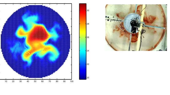
Simulations of laboratory experiments
Figure1.13shows MITgcm being used to simulate a laboratory experiment inquiring into the dynamics of the Antarctic Circumpolar Current (ACC). An initially homogeneous tank of water (1min diameter) is driven from its free surface by a rotating heated disk. The combined action of mechanical and thermal
1.2. ILLUSTRATIONS OF THE MODEL IN ACTION 21 50 100 150 200 250 0 100 200 300 400 500 600 700 (a) Simulation Longitude Day (from 1/1/1997) 50 100 150 200 250 (b) Assimilation Longitude −30 −20 −10 0 10 20 30 50 100 150 200 250 Longitude (c) Observation (T/P) cm
Figure 1.11: Top panel shows circulation patterns from a multi-year, global circulation simulation con-strained by Topex altimeter data and WOCE cruise observations. Bottom panel shows the equatorial sea-surface height in unconstrained (left), constrained (middle) simulations and in observations. This output is from a higher resolution, shorter duration experiment with equatorially enhanced grid spacing.
26.8
26.2
25.5
26.5
27
26.8
26.2
26
25.5
25.5
25.8
25
26
26.5
26.2
26.8
26.5
MITgcm air−sea O
2
flux (mol/m2/yr) with contoured potential density
150
oW
120
oW
60
oW
30
oW
0
o30
oE
60
oE
90
oE
120
oE
150
oE
180
oW
70
oS
60
oS
50
oS
40
oS
−15
−10
−5
0
5
10
15
Figure 1.12: Annual air-sea flux of oxygen (shaded) plotted along with potential density outcrops of the surface of the southern ocean from a global 1◦×1◦ integation with a telescoping grid (to 1
3
◦
) at the equator.
1.3. CONTINUOUS EQUATIONS IN ‘R’ COORDINATES 23 20 22 24 26 28 30 10 20 30 40 50 60 70 80 90 100 10 20 30 40 50 60 70 80 90 100
Figure 1.13: A numerical simulation (left) of a 1m diameter laboratory experiment (right) using MITgcm.
forcing creates a lens of fluid which becomes baroclinically unstable. The stratification and depth of pen-etration of the lens is arrested by its instability in a process analogous to that which sets the stratification of the ACC.
1.3
Continuous equations in ‘r’ coordinates
To render atmosphere and ocean models from one dynamical core we exploit ‘isomorphisms’ between equation sets that govern the evolution of the respective fluids - see figure 1.14. One system of hydro-dynamical equations is written down and encoded. The model variables have different interpretations depending on whether the atmosphere or ocean is being studied. Thus, for example, the vertical coordi-nate ‘r’ is interpreted as pressure,p, if we are modeling the atmosphere (right hand side of figure1.14) and height,z, if we are modeling the ocean (left hand side of figure1.14).
The state of the fluid at any time is characterized by the distribution of velocity~v, active tracersθ andS, a ‘geopotential’φ and density ρ=ρ(θ, S, p) which may depend on θ, S, and p. The equations that govern the evolution of these fields, obtained by applying the laws of classical mechanics and ther-modynamics to a Boussinesq, Navier-Stokes fluid are, written in terms of a generic vertical coordinate, r, so that the appropriate kinematic boundary conditions can be applied isomorphically see figure1.15.
D ~vh Dt + 2Ω~ ×~v h+∇hφ=Fv~h horizontal mtm (1.1) Dr˙ Dt +bk· 2~Ω×~v+∂φ ∂r +b=Fr˙ vertical mtm (1.2) ∇h·~vh+ ∂r˙ ∂r = 0 continuity (1.3)
Figure 1.14: Isomorphic equation sets used for atmosphere (right) and ocean (left).
MIT Climate Modeling Initiative
Z-P Isomorphism
z
p
ω
=0
ω
w
Figure 1.15: Vertical coordinates and kinematic boundary conditions for atmosphere (top) and ocean (bottom).
1.3. CONTINUOUS EQUATIONS IN ‘R’ COORDINATES 25 b=b(θ, S, r) equation of state (1.4) Dθ Dt =Qθ potential temperature (1.5) DS Dt =QS humidity/salinity (1.6) Here:
r is the vertical coordinate
D Dt =
∂
∂t+~v· ∇is the total derivative
∇=∇h+bk∂
∂r is the ‘grad’ operator
with∇h operating in the horizontal and bk∂r∂ operating in the vertical, wherebk is a unit vector in the vertical t is time ~ v= (u, v,r˙) = (~vh,r˙) is the velocity φis the ‘pressure’/‘geopotential’ ~
Ω is the Earth’s rotation
bis the ‘buoyancy’
θ is potential temperature
S is specific humidity in the atmosphere; salinity in the ocean
F~v are forcing and dissipation of~v
Qθare forcing and dissipation of θ
QS are forcing and dissipation ofS
TheF′sandQ′sare provided by ‘physics’ and forcing packages for atmosphere and ocean. These are
1.3.1
Kinematic Boundary conditions
1.3.1.1 vertical
at fixed and movingrsurfaces we set (see figure1.15): ˙
r= 0 atr=Rf ixed(x, y) (ocean bottom, top of the atmosphere) (1.7)
˙ r= Dr
Dt atr=Rmoving (ocean surface,bottom of the atmosphere) (1.8) Here
Rmoving =Ro+η
where Ro(x, y) is the ‘r−value’ (height or pressure, depending on whether we are in the atmosphere or ocean) of the ‘moving surface’ in the resting fluid andη is the departure fromRo(x, y) in the presence of motion.
1.3.1.2 horizontal
~v·~n= 0 (1.9)
where~nis the normal to a solid boundary.
1.3.2
Atmosphere
In the atmosphere, (see figure1.15), we interpret:
r=pis the pressure (1.10)
˙ r=Dp
Dt =ωis the vertical velocity inpcoordinates (1.11)
φ=g z is the geopotential height (1.12)
b=∂Π
∂pθis the buoyancy (1.13)
θ=T(pc p)
κ is potential temperature (1.14)
S=q, is the specific humidity (1.15)
where
T is absolute temperature pis the pressure
zis the height of the pressure surface gis the acceleration due to gravity
In the above the ideal gas law, p = ρRT, has been expressed in terms of the Exner function Π(p) given by (see Appendix Atmosphere)
Π(p) =cp(
p pc
)κ (1.16)
wherepc is a reference pressure andκ=R/cp withR the gas constant andcp the specific heat of air at constant pressure.
1.3. CONTINUOUS EQUATIONS IN ‘R’ COORDINATES 27
Rf ixed=ptop= 0
In a resting atmosphere the elevation of the mountains at the bottom is given by Rmoving =Ro(x, y) =po(x, y)
i.e. the (hydrostatic) pressure at the top of the mountains in a resting atmosphere. The boundary conditions at top and bottom are given by:
ω= 0 at r=Rf ixed (top of the atmosphere) (1.17)
ω = Dps
Dt ; atr=Rmoving (bottom of the atmosphere) (1.18) Then the (hydrostatic form of) equations (1.1-1.6) yields a consistent set of atmospheric equations which, for convenience, are written out inpcoordinates in Appendix Atmosphere - see eqs(1.59).
1.3.3
Ocean
In the ocean we interpret:
r = z is the height (1.19)
˙
r = Dz
Dt =wis the vertical velocity (1.20)
φ = p ρc is the pressure (1.21) b(θ, S, r) = g ρc (ρ(θ, S, r)−ρc) is the buoyancy (1.22)
whereρc is a fixed reference density of water andgis the acceleration due to gravity. In the above
At the bottom of the ocean: Rf ixed(x, y) =−H(x, y). The surface of the ocean is given by: Rmoving=η
The position of the resting free surface of the ocean is given byRo=Zo= 0. Boundary conditions are:
w = 0 atr=Rf ixed (ocean bottom) (1.23)
w = Dη
Dt atr=Rmoving =η (ocean surface) (1.24) whereη is the elevation of the free surface.
Then equations (1.1-1.6) yield a consistent set of oceanic equations which, for convenience, are written out inzcoordinates in Appendix Ocean - see eqs(1.99) to (1.104).
1.3.4
Hydrostatic, Quasi-hydrostatic, Quasi-nonhydrostatic and Non-hydrostatic
forms
Let us separateφin to surface, hydrostatic and non-hydrostatic terms:
φ(x, y, r) =φs(x, y) +φhyd(x, y, r) +φnh(x, y, r) (1.25) and write eq(1.1) in the form:
∂ ~vh
∂t +∇hφs+∇hφhyd+ǫnh∇hφnh =G~~vh (1.26)
∂φhyd
ǫnh
∂r˙ ∂t +
∂φnh
∂r =Gr˙ (1.28)
Hereǫnh is a non-hydrostatic parameter. TheG~~v, Gr˙
in eq(1.26) and (1.28) represent advective, metric and Coriolis terms in the momentum equations. In spherical coordinates they take the form1 - see Marshall et al 1997a for a full discussion:
Gu=−~v.∇u −nur˙ r − uvtanϕ r o −−2Ωvsinϕ+ 2Ω ˙rcosϕ +Fu advection metric Coriolis Forcing/Dissipation (1.29) Gv =−~v.∇v −nvr˙ r − u2tanϕ r o − {−2Ωusinϕ} +Fv advection metric Coriolis Forcing/Dissipation (1.30) Gr˙ =−~v.∇r˙ +nu2+v2 r o +2Ωucosϕ Fr˙ advection metric Coriolis Forcing/Dissipation (1.31)
In the above ‘r’ is the distance from the center of the earth and ‘ϕ’ is latitude.
Grad and div operators in spherical coordinates are defined in appendix OPERATORS.
1.3.4.1 Shallow atmosphere approximation
Most models are based on the ‘hydrostatic primitive equations’ (HPE’s) in which the vertical momentum equation is reduced to a statement of hydrostatic balance and the ‘traditional approximation’ is made in which the Coriolis force is treated approximately and the shallow atmosphere approximation is made. MITgcm need not make the ‘traditional approximation’. To be able to support consistent non-hydrostatic forms the shallow atmosphere approximation can be relaxed - when dividing through byrin, for example, (1.29), we do not replacerbya, the radius of the earth.
1.3.4.2 Hydrostatic and quasi-hydrostatic forms These are discussed at length in Marshall et al (1997a).
In the ‘hydrostatic primitive equations’ (HPE) all the underlined terms in Eqs. (1.29 →1.31) are neglected and ‘r’ is replaced by ‘a’, the mean radius of the earth. Once the pressure is found at one level - e.g. by inverting a 2-d Elliptic equation for φs at r=Rmoving - the pressure can be computed at all other levels by integration of the hydrostatic relation, eq(1.27).
In the ‘quasi-hydrostatic’ equations (QH)strict balance between gravity and vertical pressure gradi-ents is not imposed. The 2ΩucosϕCoriolis term are not neglected and are balanced by a non-hydrostatic contribution to the pressure field: only the terms underlined twice in Eqs. (1.29→1.31) are set to zero and, simultaneously, the shallow atmosphere approximation is relaxed. InQHall the metric terms are retained and the full variation of the radial position of a particle monitored. TheQHvertical momentum equation (1.28) becomes:
∂φnh
∂r = 2Ωucosϕ making a small correction to the hydrostatic pressure.
1In the hydrostatic primitive equations (HPE) all underlined terms in (1.29), (1.30) and (1.31) are omitted; the singly-underlined terms are included in the quasi-hydrostatic model (QH). The fully non-hydrostatic model (NH) includes all terms.
1.3. CONTINUOUS EQUATIONS IN ‘R’ COORDINATES 29
QH has good energetic credentials - they are the same as forHPE. Importantly, however, it has the same angular momentum principle as the full non-hydrostatic model (NH)- see Marshall et.al., 1997a. As inHPE only a 2-d elliptic problem need be solved.
1.3.4.3 Non-hydrostatic and quasi-nonhydrostatic forms
MITgcm presently supports a full non-hydrostatic ocean isomorph, but only a quasi-non-hydrostatic atmospheric isomorph.
Non-hydrostatic Ocean In the non-hydrostatic ocean model all terms in equations Eqs.(1.29 →
1.31) are retained. A three dimensional elliptic equation must be solved subject to Neumann boundary conditions (see below). It is important to note that use of the full NH does not admit any new ‘fast’ waves in to the system - the incompressible condition eq(1.3) has already filtered out acoustic modes. It does, however, ensure that the gravity waves are treated accurately with an exact dispersion relation. The NHset has a complete angular momentum principle and consistent energetics - see White and Bromley, 1995; Marshall et.al. 1997a.
Quasi-nonhydrostatic Atmosphere In the non-hydrostatic version of our atmospheric model we approximate ˙r in the vertical momentum eqs(1.28) and (1.30) (but only here) by:
˙ r=Dp Dt = 1 g Dφ Dt (1.32)
wherephy is the hydrostatic pressure.
1.3.4.4 Summary of equation sets supported by model
Atmosphere Hydrostatic, and quasi-hydrostatic and quasi non-hydrostatic forms of the compressible non-Boussinesq equations inp−coordinates are supported.
Hydrostatic and quasi-hydrostatic The hydrostatic set is written out inp−coordinates in ap-pendix Atmosphere - see eq(1.59).
Quasi-nonhydrostatic A quasi-nonhydrostatic form is also supported. Ocean
Hydrostatic and quasi-hydrostatic Hydrostatic, and quasi-hydrostatic forms of the incompress-ible Boussinesq equations inz−coordinates are supported.
Non-hydrostatic Non-hydrostatic forms of the incompressible Boussinesq equations inz− coordi-nates are supported - see eqs(1.99) to (1.104).
1.3.5
Solution strategy
The method of solution employed in theHPE,QHand NHmodels is summarized in Figure1.17. Under all dynamics, a 2-d elliptic equation is first solved to find the surface pressure and the hydrostatic pressure at any level computed from the weight of fluid above. Under HPE and QH dynamics, the horizontal momentum equations are then stepped forward and ˙rfound from continuity. UnderNHdynamics a 3-d elliptic equation must be solved for the non-hydrostatic pressure before stepping forward the horizontal momentum equations; ˙ris found by stepping forward the vertical momentum equation.
There is no penalty in implementing QH overHPE except, of course, some complication that goes with the inclusion of cosϕ Coriolis terms and the relaxation of the shallow atmosphere approximation. But this leads to negligible increase in computation. InNH, in contrast, one additional elliptic equation - a three-dimensional one - must be inverted for pnh. However the ‘overhead’ of the NH model is essentially negligible in the hydrostatic limit (see detailed discussion in Marshall et al, 1997) resulting in a non-hydrostatic algorithm that, in the hydrostatic limit, is as computationally economic as theHPEs.
1.3. CONTINUOUS EQUATIONS IN ‘R’ COORDINATES 31
Figure 1.17: Basic solution strategy in MITgcm. HPE andQHforms diagnose the vertical velocity, in NHa prognostic equation for the vertical velocity is integrated.
1.3.6
Finding the pressure field
Unlike the prognostic variables u, v, w, θ and S, the pressure field must be obtained diagnostically. We proceed, as before, by dividing the total (pressure/geo) potential in to three parts, a surface part, φs(x, y), a hydrostatic partφhyd(x, y, r) and a non-hydrostatic partφnh(x, y, r), as in (1.25), and writing the momentum equation as in (1.26).
1.3.6.1 Hydrostatic pressure
Hydrostatic pressure is obtained by integrating (1.27) vertically fromr=Ro where φhyd(r =Ro) = 0, to yield: Z Ro r ∂φhyd ∂r dr= [φhyd] Ro r = Z Ro r − bdr and so φhyd(x, y, r) = Z Ro r bdr (1.33)
The model can be easily modified to accommodate a loading term (e.g atmospheric pressure pushing down on the ocean’s surface) by setting:
φhyd(r=Ro) =loading (1.34)
1.3.6.2 Surface pressure
The surface pressure equation can be obtained by integrating continuity, (1.3), vertically fromr=Rf ixed tor=Rmoving Z Rmoving Rf ixed (∇h·~vh+∂rr˙)dr= 0 Thus: ∂η ∂t +~v.∇η+ Z Rmoving Rf ixed ∇h·~vhdr= 0
where η = Rmoving −Ro is the free-surface r-anomaly in units of r. The above can be rearranged to yield, using Leibnitz’s theorem:
∂η ∂t +∇h· Z Rmoving Rf ixed ~ vhdr= source (1.35)
where we have incorporated a source term.
Whether φis pressure (ocean model,p/ρc) or geopotential (atmospheric model), in (1.26), the hori-zontal gradient term can be written
∇hφs=∇h(bsη) (1.36)
wherebsis the buoyancy at the surface.
In the hydrostatic limit (ǫnh = 0), equations (1.26), (1.35) and (1.36) can be solved by inverting a 2-d elliptic equation forφs as described in Chapter 2. Both ‘free surface’ and ‘rigid lid’ approaches are available.
1.3.6.3 Non-hydrostatic pressure
Taking the horizontal divergence of (1.26) and adding ∂
∂r of (1.28), invoking the continuity equation (1.3), we deduce that:
∇23φnh =∇. ~G~v− ∇2hφs+∇2φhyd=∇.~F (1.37) For a given rhs this 3-d elliptic equation must be inverted for φnh subject to appropriate choice of boundary conditions. This method is usually called The Pressure Method [Harlow and Welch, 1965; Williams, 1969; Potter, 1976]. In the hydrostatic primitive equations case (HPE), the 3-d problem does not need to be solved.
Boundary Conditions We apply the condition of no normal flow through all solid boundaries - the coasts (in the ocean) and the bottom:
~
v.bn= 0 (1.38)
wherebnis a vector of unit length normal to the boundary. The kinematic condition (1.38) is also applied to the vertical velocity atr=Rmoving. No-slip (vT = 0) or slip (∂vT/∂n= 0) conditions are employed on the tangential component of velocity, vT, at all solid boundaries, depending on the form chosen for the dissipative terms in the momentum equations - see below.
Eq.(1.38) implies, making use of (1.26), that:
b
n.∇φnh=bn.~F (1.39)
where
~
F=G~~v−(∇hφs+∇φhyd)
presenting inhomogeneous Neumann boundary conditions to the Elliptic problem (1.37). As shown, for example, by Williams (1969), one can exploit classical 3D potential theory and, by introducing an appropriately chosenδ-function sheet of ‘source-charge’, replace the inhomogeneous boundary condition on pressure by a homogeneous one. The source term rhs in (1.37) is the divergence of the vector F~. By simultaneously setting bn.~F = 0 andbn.∇φnh = 0 on the boundary the following self-consistent but simpler homogenized Elliptic problem is obtained:
∇2φnh=∇.~Fe
where F~e is a modified F~ such that F~e.bn= 0. As is implied by (1.39) the modified boundary condition becomes:
b
1.3. CONTINUOUS EQUATIONS IN ‘R’ COORDINATES 33
If the flow is ‘close’ to hydrostatic balance then the 3-d inversion converges rapidly because φnh is then only a small correction to the hydrostatic pressure field (see the discussion in Marshall et al, a,b).
The solutionφnh to (1.37) and (1.39) does not vanish atr =Rmoving, and so refines the pressure there.
1.3.7
Forcing/dissipation
1.3.7.1 Forcing
The forcing termsF on the rhs of the equations are provided by ‘physics packages’ and forcing packages. These are described later on.
1.3.7.2 Dissipation
Momentum Many forms of momentum dissipation are available in the model. Laplacian and bihar-monic frictions are commonly used:
DV =Ah∇2hv+Av
∂2v
∂z2 +A4∇ 4
hv (1.41)
where Ah and Av are (constant) horizontal and vertical viscosity coefficients and A4 is the horizontal
coefficient for biharmonic friction. These coefficients are the same for all velocity components.
Tracers The mixing terms for the temperature and salinity equations have a similar form to that of momentum except that the diffusion tensor can be non-diagonal and have varying coefficients.
DT,S=∇.[K∇(T, S)] +K4∇4h(T, S) (1.42) where K is the diffusion tensor and the K4 horizontal coefficient for biharmonic diffusion. In the
simplest case where the subgrid-scale fluxes of heat and salt are parameterized with constant horizontal and vertical diffusion coefficients,K, reduces to a diagonal matrix with constant coefficients:
K= K0h K0h 00 0 0 Kv (1.43)
whereKh and Kv are the horizontal and vertical diffusion coefficients. These coefficients are the same for all tracers (temperature, salinity ... ).
1.3.8
Vector invariant form
For some purposes it is advantageous to write momentum advection in eq(1.1) and (1.2) in the (so-called) ‘vector invariant’ form:
D~v Dt = ∂~v ∂t + (∇ ×~v)×~v+∇ 1 2(~v·~v) (1.44)
This permits alternative numerical treatments of the non-linear terms based on their representation as a vorticity flux. Because gradients of coordinate vectors no longer appear on the rhs of (1.44), explicit representation of the metric terms in (1.29), (1.30) and (1.31), can be avoided: information about the geometry is contained in the areas and lengths of the volumes used to discretize the model.
1.3.9
Adjoint
1.4
Appendix ATMOSPHERE
1.4.1
Hydrostatic Primitive Equations for the Atmosphere in pressure
coor-dinates
The hydrostatic primitive equations (HPEs) in p-coordinates are: D~vh Dt +fkˆ×~vh+∇pφ = F~ (1.45) ∂φ ∂p +α = 0 (1.46) ∇p·~vh+ ∂ω ∂p = 0 (1.47) pα = RT (1.48) cv DT Dt +p Dα Dt = Q (1.49)
where~vh= (u, v,0) is the ‘horizontal’ (on pressure surfaces) component of velocity, D Dt=
∂
∂t+~vh·∇p+ω ∂ ∂p is the total derivative,f = 2Ω sinϕis the Coriolis parameter,φ=gz is the geopotential,α= 1/ρ is the specific volume,ω = DpDt is the vertical velocity in thep−coordinate. Equation(1.49) is the first law of thermodynamics where internal energye=cvT,T is temperature,Qis the rate of heating per unit mass andpDαDt is the work done by the fluid in compressing.
It is convenient to cast the heat equation in terms of potential temperature θ so that it looks more like a generic conservation law. Differentiating (1.48) we get:
pDα Dt +α Dp Dt =R DT Dt
which, when added to the heat equation (1.49) and usingcp=cv+R, gives:
cp
DT Dt −α
Dp
Dt =Q (1.50)
Potential temperature is defined:
θ=T(pc p)
κ (1.51)
where pc is a reference pressure andκ=R/cp. For convenience we will make use of the Exner function Π(p) which defined by:
Π(p) =cp(
p pc
)κ (1.52)
The following relations will be useful and are easily expressed in terms of the Exner function:
cpT = Πθ ; ∂Π ∂p = κΠ p ; α= κΠθ p = ∂ Π ∂p θ ; DΠ Dt = ∂Π ∂p Dp Dt whereb=∂∂pΠθis the buoyancy.
The heat equation is obtained by noting that
cp DT Dt = D(Πθ) Dt = Π Dθ Dt +θ DΠ Dt = Π Dθ Dt +α Dp Dt and on substituting into (1.50) gives:
ΠDθ
Dt =Q (1.53)
which is in conservative form.
1.4. APPENDIX ATMOSPHERE 35
1.4.1.1 Boundary conditions
The upper and lower boundary conditions are :
at the top: p= 0 ,ω= Dp
Dt = 0 (1.54)
at the surface: p=ps ,φ=φtopo =g Ztopo (1.55)
Inp-coordinates, the upper boundary acts like a solid boundary (ω= 0); inz-coordinates and the lower boundary is analogous to a free surface (φis imposed andω6= 0).
1.4.1.2 Splitting the geo-potential
For the purposes of initialization and reducing round-off errors, the model deals with perturbations from reference (or “standard”) profiles. For example, the hydrostatic geopotential associated with the resting atmosphere is not dynamically relevant and can therefore be subtracted from the equations. The equations written in terms of perturbations are obtained by substituting the following definitions into the previous model equations:
θ = θo+θ′ (1.56)
α = αo+α′ (1.57)
φ = φo+φ′ (1.58)
The reference state (indicated by subscript “0”) corresponds to horizontally homogeneous atmosphere at rest (θo, αo, φo) with surface pressurepo(x, y) that satisfiesφo(po) =g Ztopo, defined:
θo(p) = fn(p) αo(p) = Πpθo φo(p) = φtopo− Z p p0 αodp
The final form of the HPE’s in p coordinates is then:
D~vh Dt +fkˆ×~vh+∇pφ ′ = ~ F (1.59) ∂φ′ ∂p +α ′ = 0 (1.60) ∇p·~vh+ ∂ω ∂p = 0 (1.61) ∂Π ∂pθ ′ = α′ (1.62) Dθ Dt = Q Π (1.63)
1.5
Appendix OCEAN
1.5.1
Equations of motion for the ocean
We review here the method by which the standard (Boussinesq, incompressible) HPE’s for the ocean written in z-coordinates are obtained. The non-Boussinesq equations for oceanic motion are:
D~vh Dt +fkˆ×~vh+ 1 ρ∇zp = F~ (1.64) ǫnh Dw Dt +g+ 1 ρ ∂p ∂z = ǫnhFw (1.65) 1 ρ Dρ Dt +∇z·~vh+ ∂w ∂z = 0 (1.66) ρ = ρ(θ, S, p) (1.67) Dθ Dt = Qθ (1.68) DS Dt = Qs (1.69)
These equations permit acoustics modes, inertia-gravity waves, non-hydrostatic motions, a geostrophic (Rossby) mode and a thermohaline mode. As written, they cannot be integrated forward consistently -if we step ρforward in (1.66), the answer will not be consistent with that obtained by stepping (1.68) and (1.69) and then using (1.67) to yieldρ. It is therefore necessary to manipulate the system as follows. Differentiating the EOS (equation of state) gives:
Dρ Dt = ∂ρ ∂θ S,pDθDt + ∂ρ ∂S θ,pDSDt + ∂ρ ∂p θ,S DpDt (1.70) Note that ∂ρ∂p = c12
s is the reciprocal of the sound speed (cs) squared. Substituting into1.66gives:
1 ρc2
s
Dp
Dt +∇z·~v+∂zw≈0 (1.71)
where we have used an approximation sign to indicate that we have assumed adiabatic motion, dropping the DθDt and DSDt. Replacing1.66with1.71yields a system that can be explicitly integrated forward:
D~vh Dt +fkˆ×~vh+ 1 ρ∇zp = F~ (1.72) ǫnh Dw Dt +g+ 1 ρ ∂p ∂z = ǫnhFw (1.73) 1 ρc2 s Dp Dt +∇z·~vh+ ∂w ∂z = 0 (1.74) ρ = ρ(θ, S, p) (1.75) Dθ Dt = Qθ (1.76) DS Dt = Qs (1.77)
1.5.1.1 Compressible z-coordinate equations
Here we linearize the acoustic modes by replacing ρ with ρo(z) wherever it appears in a product (ie. non-linear term) - this is the ‘Boussinesq assumption’. The only term that then retains the full variation
1.5. APPENDIX OCEAN 37
inρis the gravitational acceleration: D~vh Dt +fkˆ×~vh+ 1 ρo∇zp = ~ F (1.78) ǫnh Dw Dt + gρ ρo + 1 ρo ∂p ∂z = ǫnhFw (1.79) 1 ρoc2s Dp Dt +∇z·~vh+ ∂w ∂z = 0 (1.80) ρ = ρ(θ, S, p) (1.81) Dθ Dt = Qθ (1.82) DS Dt = Qs (1.83)
These equations still retain acoustic modes. But, because the “compressible” terms are linearized, the pressure equation 1.80 can be integrated implicitly with ease (the time-dependent term appears as a Helmholtz term in the non-hydrostatic pressure equation). These are thetruly compressible Boussinesq equations. Note that the EOS must have the same pressure dependency as the linearized pressure term, ie. ∂ρ∂p
θ,S=
1
c2
s, for consistency.
1.5.1.2 ‘Anelastic’ z-coordinate equations
The anelastic approximation filters the acoustic mode by removing the time-dependency in the continuity (now pressure-) equation (1.80). This could be done simply by noting that DpDt ≈ −gρoDzDt =−gρow, but this leads to an inconsistency between continuity and EOS. A better solution is to change the dependency on pressure in the EOS by splitting the pressure into a reference function of height and a perturbation:
ρ=ρ(θ, S, po(z) +ǫsp′)
Remembering that the termDpDt in continuity comes from differentiating the EOS, the continuity equation then becomes: 1 ρoc2s Dp o Dt +ǫs Dp′ Dt +∇z·~vh+ ∂w ∂z = 0
If the time- and space-scales of the motions of interest are longer than those of acoustic modes, then Dp′
Dt << ( Dpo
Dt,∇ ·~vh) in the continuity equations and ∂ρ ∂p θ,S Dp′ Dt << ∂ρ ∂p θ,S Dpo Dt in the EOS (1.70). Thus we set ǫs = 0, removing the dependency on p′ in the continuity equation and EOS. Expanding Dpo(z)
Dt =−gρow then leads to the anelastic continuity equation:
∇z·~vh+ ∂w ∂z − g c2 s w= 0 (1.84)
A slightly different route leads to the quasi-Boussinesq continuity equation where we use the scaling ∂ρ′ ∂t +∇3·ρ′~v<<∇3·ρo~vyielding: ∇z·~vh+ 1 ρo ∂(ρow) ∂z = 0 (1.85)
Equations1.84and1.85are in fact the same equation if: 1 ρo ∂ρo ∂z = −g c2 s (1.86)
Again, note that ifρo is evaluated from prescribedθo and So profiles, then the EOS dependency on po and the term cg2
or ‘anelastic’ equations for the ocean are then: D~vh Dt +fkˆ×~vh+ 1 ρo∇z p = F~ (1.87) ǫnh Dw Dt + gρ ρo + 1 ρo ∂p ∂z = ǫnhFw (1.88) ∇z·~vh+ 1 ρo ∂(ρow) ∂z = 0 (1.89) ρ = ρ(θ, S, po(z)) (1.90) Dθ Dt = Qθ (1.91) DS Dt = Qs (1.92)
1.5.1.3 Incompressible z-coordinate equations
Here, the objective is to drop the depth dependence ofρo and so, technically, to also remove the depen-dence ofρonpo. This would yield the “truly” incompressible Boussinesq equations:
D~vh Dt +fˆk×~vh+ 1 ρc∇z p = F~ (1.93) ǫnh Dw Dt + gρ ρc + 1 ρc ∂p ∂z = ǫnhFw (1.94) ∇z·~vh+∂w ∂z = 0 (1.95) ρ = ρ(θ, S) (1.96) Dθ Dt = Qθ (1.97) DS Dt = Qs (1.98)
whereρc is a constant reference density of water. 1.5.1.4 Compressible non-divergent equations
The above “incompressible” equations are incompressible in both the flow and the density. In many oceanic applications, however, it is important to retain compressibility effects in the density. To do this we must split the density thus:
ρ=ρo+ρ′
We then assert that variations with depth ofρoare unimportant while the compressible effects inρ′ are:
ρo=ρc
ρ′ =ρ(θ, S, po(z))−ρo
This then yields what we can call the semi-compressible Boussinesq equations: D~vh Dt +fkˆ×~vh+ 1 ρc∇ zp′ = F~ (1.99) ǫnh Dw Dt + gρ′ ρc + 1 ρc ∂p′ ∂z = ǫnhFw (1.100) ∇z·~vh+ ∂w ∂z = 0 (1.101) ρ′ = ρ(θ, S, po(z))−ρc (1.102) Dθ Dt = Qθ (1.103) DS Dt = Qs (1.104)
1.6. APPENDIX:OPERATORS 39
Note that the hydrostatic pressure of the resting fluid, including that associated withρc, is subtracted out since it has no effect on the dynamics.
Though necessary, the assumptions that go into these equations are messy since we essentially assume a different EOS for the reference density and the perturbation density. Nevertheless, it is the hydrostatic (ǫnh = 0 form of these equations that are used throughout the ocean modeling community and referred to as the primitive equations (HPE).
1.6
Appendix:OPERATORS
1.6.1
Coordinate systems
1.6.1.1 Spherical coordinates
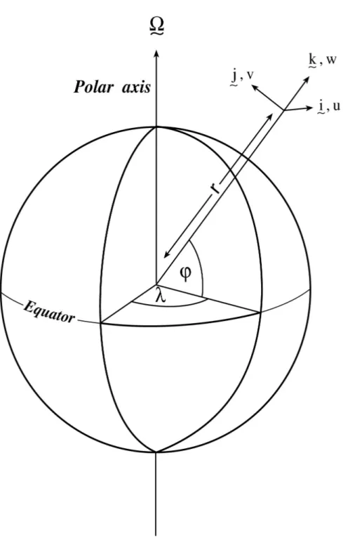
In spherical coordinates, the velocity components in the zonal, meridional and vertical direction respec-tively, are given by (see Fig.2) :
u=rcosϕDλ Dt v=rDϕ Dt ˙ r=Dr Dt
Here ϕ is the latitude, λ the longitude,r the radial distance of the particle from the center of the earth, Ω is the angular speed of rotation of the Earth andD/Dtis the total derivative.
The ‘grad’ (∇) and ‘div’ (∇·) operators are defined by, in spherical coordinates:
∇ ≡ 1 rcosϕ ∂ ∂λ, 1 r ∂ ∂ϕ, ∂ ∂r ∇ ·v ≡rcos1 ϕ ∂u ∂λ+ ∂ ∂ϕ(vcosϕ) + 1 r2 ∂ r2r˙ ∂r
Chapter 2
Discretization and Algorithm
This chapter lays out the numerical schemes that are employed in the core MITgcm algorithm. Whenever possible links are made to actual program code in the MITgcm implementation. The chapter begins with a discussion of the temporal discretization used in MITgcm. This discussion is followed by sections that describe the spatial discretization. The schemes employed for momentum terms are described first, afterwards the schemes that apply to passive and dynamically active tracers are described.
2.1
Notation
Because of the particularity of the vertical direction in stratified fluid context, in this chapter, the vector notations are mostly used for the horizontal component: the horizontal part of a vector is simply written ~v(instead ofvh or~vh in chaper 1) and a 3.D vector is simply written~v (instead of~v in chapter 1).
The notations we use to describe the discrete formulation of the model are summarized hereafter: general notation:
∆x,∆y,∆rgrid spacing in X,Y,R directions.
Ac, Aw, As, Aζ : horizontal area of a grid cell surroundingθ, u, v, ζ point.
Vu,Vv,Vw,Vθ : Volume of the grid box surroundingu, v, w, θpoint;
i, j, k: current index relative to X,Y,R directions; basic operator:
δi : δiΦ = Φi+1/2−Φi−1/2 −i : Φi= (Φ
i+1/2+ Φi−1/2)/2
δx : δxΦ =∆1xδiΦ
∇= horizontal gradient operator : ∇Φ ={δxΦ, δyΦ}
∇·= horizontal divergence operator : ∇ ·~f = A1{δi∆yfx+δj∆xfy}
∇2 = horizontal Laplacian operator : ∇2Φ =∇ · ∇Φ
2.2
Time-stepping
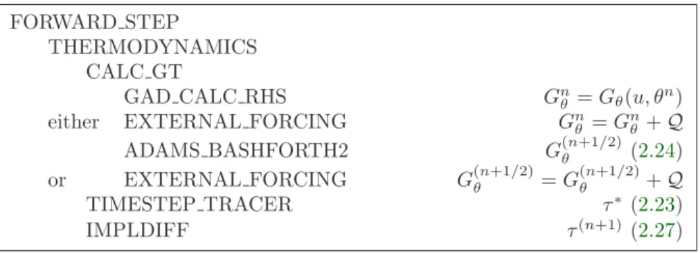
The equations of motion integrated by the model involve four prognostic equations for flow,uandv, tem-perature,θ, and salt/moisture,S, and three diagnostic equations for vertical flow,w, density/buoyancy, ρ/b, and pressure/geo-potential,φhyd. In addition, the surface pressure or height may by described by either a prognostic or diagnostic equation and if non-hydrostatics terms are included then a diagnostic equation for non-hydrostatic pressure is also solved. The combination of prognostic and diagnostic equa-tions requires a model algorithm that can march forward prognostic variables while satisfying constraints imposed by diagnostic equations.
Since the model comes in several flavors and formulation, it would be confusing to present the model algorithm exactly as written into code along with all the switches and optional terms. Instead, we present the algorithm for each of the basic formulations which are:
( )
u,v
G
(n+½)
u,v
n+1
∆
2
η
=
∆
.
u
v
*
*
∆
(n+1) t
∆
time
n t
n
*
u,v
u,v
Figure 2.1: A schematic of the evolution in time of the pressure method algorithm. A prediction for the flow variables at time leveln+ 1 is made based only on the explicit terms,G(n+1/
2), and denotedu∗,v∗.
Next, a pressure field is found such thatun+1,vn+1 will be non-divergent. Conceptually, the∗quantities
exist at time leveln+ 1 but they are intermediate and only temporary.
1. the semi-implicit pressure method for hydrostatic equations with a rigid-lid, variables co-located in time and with Adams-Bashforth time-stepping,
2. as1. but with an implicit linear free-surface, 3. as1. or2. but with variables staggered in time, 4. as1. or2. but with non-hydrostatic terms included, 5. as2. or3. but with non-linear free-surface.
In all the above configurations it is also possible to substitute the Adams-Bashforth with an alter-native time-stepping scheme for terms evaluated explicitly in time. Since the over-arching algorithm is independent of the particular time-stepping scheme chosen we will describe first the over-arching algo-rithm, known as the pressure method, with a rigid-lid model in section2.3. This algorithm is essentially unchanged, apart for some coefficients, when the rigid lid assumption is replaced with a linearized implicit free-surface, described in section2.4. These two flavors of the pressure-method encompass all formulations of the model as it exists today. The integration of explicit in time terms is out-lined in section2.5and put into the context of the overall algorithm in sections2.7and 2.8. Inclusion of non-hydrostatic terms requires applying the pressure method in three dimensions instead of two and this algorithm modifica-tion is described in secmodifica-tion2.9. Finally, the free-surface equation may be treated more exactly, including non-linear terms, and this is described in section2.10.2.
2.3
Pressure method with rigid-lid
The horizontal momentum and continuity equations for the ocean (1.99and1.101), or for the atmosphere (1.45and1.47), can be summarized by:
∂tu+g∂xη = Gu (2.1)
∂tv+g∂yη = Gv (2.2)
∂xu+∂yv+∂zw = 0 (2.3)
where we are adopting the oceanic notation for brevity. All terms in the momentum equations, except for surface pressure gradient, are encapsulated in theGvector. The continuity equation, when integrated
2.3. PRESSURE METHOD WITH RIGID-LID 43
FORWARD STEP
DYNAMICS
TIMESTEP u∗,v∗ (2.8,2.9)
SOLVE FOR PRESSURE
CALC DIV GHAT Hcu∗,Hvb∗(2.10)
CG2D ηn+1(2.10)
MOMENTUM CORRECTION STEP
CALC GRAD PHI SURF ∇ηn+1
CORRECTION STEP un+1,vn+1 (2.11,2.12)
Figure 2.2: Calling tree for the pressure method algorithm (FORWARD STEP)
over the fluid depth,H, and with the rigid-lid/no normal flow boundary conditions applied, becomes:
∂xHbu+∂yHvb= 0 (2.4)
Here,Hub=RHudzis the depth integral ofu, similarly forHbv. The rigid-lid approximation setsw= 0 at the lid so that it does not move but allows a pressure to be exerted on the fluid by the lid. The horizontal momentum equations and vertically integrated continuity equation are be discretized in time and space as follows:
un+1+ ∆tg∂
xηn+1 = un+ ∆tG(un+1/2) (2.5)
vn+1+ ∆tg∂yηn+1 = vn+ ∆tG(vn+1/2) (2.6)
∂xHudn+1+∂yHvdn+1 = 0 (2.7)
As written here, terms on the LHS all involve time leveln+ 1 and are referred to as implicit; the implicit backward time stepping scheme is being used. All other terms in the RHS are explicit in time. The thermodynamic quantities are integrated forward in time in parallel with the flow and will be discussed later. For the purposes of describing the pressure method it suffices to say that the hydrostatic pressure gradient is explicit and so can be included in the vectorG.
Substituting the two momentum equations into the depth integrated continuity equation eliminates un+1andvn+1yielding an elliptic equation forηn+1. Equations2.5,2.6and2.7can then be re-arranged
as follows: u∗ = un+ ∆tG(n+1/2) u (2.8) v∗ = vn+ ∆tG(vn+1/2) (2.9) ∂x∆tgH∂xηn+1+∂y∆tgH∂yηn+1 = ∂xHcu∗+∂yHvb∗ (2.10) un+1 = u∗−∆tg∂xηn+1 (2.11) vn+1 = v∗−∆tg∂yηn+1 (2.12) Equations2.8 to2.12, solved sequentially, represent the pressure method algorithm used in the model. The essence of the pressure method lies in the fact that any explicit prediction for the flow would lead to a divergence flow field so a pressure field must be found that keeps the flow non-divergent over each step of the integration. The particular location in time of the pressure field is somewhat ambiguous; in Fig.2.1 we depicted as co-located with the future flow field (time leveln+ 1) but it could equally have been drawn as staggered in time with the flow.
The correspondence to the code is as follows:
• the prognostic phase, equations2.8 and2.9, stepping forwardun and vn to u∗ and v∗ is coded in
TIMESTEP()
• the vertical integration,Hcu∗andHvb∗, divergence and inversion of the elliptic operator in equation
2.10is coded in SOLVE FOR PRESSURE()
• finally, the new flow field at time level n+ 1 given by equations 2.11 and 2.12 is calculated in
The calling tree for these routines is given in Fig.2.2.
In general, the horizontal momentum time-stepping can contain some terms that are treated implicitly in time, such as the vertical viscosity when using the backward time-stepping scheme (implicitViscosity =.TRUE.). The method used to solve those implicit terms is provided in section2.6, and modifies equa-tions2.5and2.6to give:
un+1−∆t∂zAv∂zun+1+ ∆tg∂xηn+1 = un+ ∆tG(un+1/2) (2.13)
vn+1−∆t∂zAv∂zvn+1+ ∆tg∂yηn+1 = vn+ ∆tG(vn+1/2) (2.14)
2.4
Pressure method with implicit linear free-surface
The rigid-lid approximation filters out external gravity waves subsequently modifying the dispersion relation of barotropic Rossby waves. The discrete form of the elliptic equation has some zero eigen-values which makes it a potentially tricky or inefficient problem to solve.
The rigid-lid approximation can be easily replaced by a linearization of the free-surface equation which can be written:
∂tη+∂xHub+∂yHbv=P−E+R (2.15) which differs from the depth integrated continuity equation with rigid-lid (2.4) by the time-dependent term and fresh-water source term.
Equation2.7in the rigid-lid pressure method is then replaced by the time discretization of2.15which is:
ηn+1+ ∆t∂xHudn+1+ ∆t∂yHvdn+1=ηn+ ∆t(P−E) (2.16) where the use of flow at time level n+ 1 makes the method implicit and backward in time. This is the preferred scheme since it still filters the fast unresolved wave motions by damping them. A centered scheme, such as Crank-Nicholson (see section2.10.1), would alias the energy of the fast modes onto slower modes of motion.
As for the rigid-lid pressure method, equations 2.5,2.6and2.16can be re-arranged as follows:
u∗ = un+ ∆tG(un+1/2) (2.17) v∗ = vn+ ∆tG(vn+1/2) (2.18) η∗ = ǫf s(ηn+ ∆t(P−E))−∆t ∂xHuc∗+∂yHvb∗ (2.19) ∂xgH∂xηn+1 + ∂ygH∂yηn+1− ǫf sηn+1 ∆t2 =− η∗ ∆t2 (2.20) un+1 = u∗−∆tg∂ xηn+1 (2.21) vn+1 = v∗−∆tg∂yηn+1 (2.22)
Equations 2.17to 2.22, solved sequentially, represent the pressure method algorithm with a backward implicit, linearized free surface. The method is still formerly a pressure method because in the limit of large ∆t the r