March 1, 2009
Support Vector Machines Explained
Tristan Fletcher
Introduction
This document has been written in an attempt to make the Support Vector Machines (SVM), initially conceived of by Cortes and Vapnik [1], as sim-ple to understand as possible for those with minimal experience of Machine Learning. It assumes basic mathematical knowledge in areas such as cal-culus, vector geometry and Lagrange multipliers. The document has been split into Theory and Application sections so that it is obvious, after the maths has been dealt with, how to actually apply the SVM for the different forms of problem that each section is centred on.
The document’s first section details the problem of classification for linearly separable data and introduces the concept of margin and the essence of SVM - margin maximization. The methodology of the SVM is then extended to data which is not fully linearly separable. Thissoft margin SVM introduces the idea of slack variables and the trade-off between maximizing the margin and minimizing the number of misclassified variables in the second section. The third section develops the concept of SVM further so that the technique can be used for regression.
The fourth section explains the other salient feature of SVM - the Kernel Trick. It explains how incorporation of this mathematical sleight of hand allows SVM to classify and regress nonlinear data.
Other than Cortes and Vapnik [1], most of this document is based on work by Cristianini and Shawe-Taylor [2], [3], Burges [4] and Bishop [5].
For any comments on or questions about this document, please contact the author through the URL on the title page.
Acknowledgments
1
Linearly Separable Binary Classification
1.1 Theory
We haveL training points, where each inputxi hasD attributes (i.e. is of dimensionalityD) and is in one of two classesyi = -1 or +1, i.e our training
data is of the form:
{xi, yi} where i= 1. . . L, yi ∈ {−1,1}, x∈ ℜD
Here we assume the data is linearly separable, meaning that we can draw a line on a graph ofx1 vs x2 separating the two classes when D= 2 and a
hyperplane on graphs ofx1, x2. . . xD for when D >2.
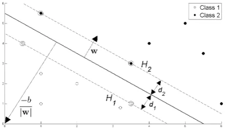
This hyperplane can be described by w·x+b= 0 where: • wis normal to the hyperplane.
• kwbk is the perpendicular distance from the hyperplane to the origin. Support Vectors are the examples closest to the separating hyperplane and the aim of Support Vector Machines (SVM) is to orientate this hyperplane in such a way as to be as far as possible from the closest members of both classes.
Figure 1: Hyperplane through two linearly separable classes
Referring to Figure 1, implementing a SVM boils down to selecting the variables wandb so that our training data can be described by:
xi·w+b≥+1 foryi = +1 (1.1)
xi·w+b≤ −1 foryi =−1 (1.2)
These equations can be combined into:
If we now just consider the points that lie closest to the separating hyper-plane, i.e. the Support Vectors (shown in circles in the diagram), then the two planesH1 and H2 that these points lie on can be described by:
xi·w+b= +1 forH1 (1.4)
xi·w+b=−1 forH2 (1.5)
Referring to Figure 1, we define d1 as being the distance from H1 to the
hyperplane and d2 from H2 to it. The hyperplane’s equidistance from H1
and H2 means that d1 =d2 - a quantity known as the SVM’s margin. In
order to orientate the hyperplane to be as far from the Support Vectors as possible, we need to maximize this margin.
Simple vector geometry shows that the margin is equal to 1
kwk and maxi-mizing it subject to the constraint in (1.3) is equivalent to finding:
minkwk such that yi(xi·w+b)−1≥0 ∀i Minimizingkwkis equivalent to minimizing 1
2kwk 2
and the use of this term makes it possible to perform Quadratic Programming (QP) optimization later on. We therefore need to find:
min1 2kwk
2
s.t. yi(xi·w+b)−1≥0 ∀i (1.6)
In order to cater for the constraints in this minimization, we need to allocate them Lagrange multipliersα, whereαi ≥0 ∀i:
We wish to find the wand bwhich minimizes, and the α which maximizes (1.9) (whilst keepingαi ≥0∀i). We can do this by differentiating LP with
Substituting (1.10) and (1.11) into (1.9) gives a new formulation which, being dependent on α, we need to maximize:
LD ≡
This new formulation LD is referred to as the Dual form of the Primary
LP. It is worth noting that the Dual form requires only the dot product of
each input vectorxi to be calculated, this is important for the Kernel Trick
described in the fourth section.
Having moved from minimizingLP to maximizing LD, we need to find:
max This is a convex quadratic optimization problem, and we run a QP solver which will return α and from (1.10) will give us w. What remains is to calculateb.
Any data point satisfying (1.11) which is a Support Vectorxs will have the
form:
WhereS denotes the set of indices of the Support Vectors. S is determined by finding the indicesi whereαi >0. Multiplying through byys and then
Instead of using an arbitrary Support Vector xs, it is better to take an average over all of the Support Vectors in S:
b= 1 Ns
X
s∈S
(ys−
X
m∈S
αmymxm·xs) (1.16)
1.2 Application
In order to use an SVM to solve a linearly separable, binary classification problem we need to:
• CreateH, whereHij =yiyjxi·xj. • Find αso that
L
X
i=1
αi−
1 2α
THα
is maximized, subject to the constraints
αi ≥0 ∀i and L
X
i=1
αiyi = 0.
This is done using a QP solver.
• Calculatew=
L
X
i=1
αiyixi.
• Determine the set of Support Vectors S by finding the indices such thatαi>0.
• Calculateb= 1
Ns X
s∈S
(ys−
X
m∈S
αmymxm·xs).
2
Binary Classification for Data that is not Fully
Linearly Separable
2.1 Theory
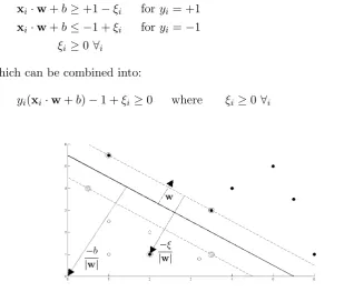
In order to extend the SVM methodology to handle data that is not fully linearly separable, we relax the constraints for (1.1) and (1.2) slightly to allow for misclassified points. This is done by introducing a positive slack variableξi, i= 1, . . . L:
xi·w+b≥+1−ξi foryi= +1 (2.1)
xi·w+b≤ −1 +ξi foryi=−1 (2.2)
ξi ≥0 ∀i (2.3)
Which can be combined into:
yi(xi·w+b)−1 +ξi ≥0 where ξi≥0 ∀i (2.4)
Figure 2: Hyperplane through two non-linearly separable classes In this soft margin SVM, data points on the incorrect side of the margin boundary have a penalty that increases with the distance from it. As we are trying to reduce the number of misclassifications, a sensible way to adapt our objective function (1.6) from previously, is to find:
min1 2kwk
2
+C
L
X
i=1
ξi s.t. yi(xi·w+b)−1 +ξi ≥0 ∀i (2.5)
with respect toα (where αi ≥0,µi ≥0 ∀i):
Differentiating with respect to w, b and ξi and setting the derivatives to zero:
Substituting these in,LD has the same form as (1.14) before. However (2.9)
2.2 Application
In order to use an SVM to solve a binary classification for data that is not fully linearly separable we need to:
• CreateH, whereHij =yiyjxi·xj.
• Choose how significantly misclassifications should be treated, by se-lecting a suitable value for the parameterC.
• Find αso that
L
X
i=1
αi−
1 2α
TH
α
is maximized, subject to the constraints
0≤αi≤ C ∀i and L
X
i=1
αiyi = 0.
This is done using a QP solver.
• Calculatew=
L
X
i=1
αiyixi.
• Determine the set of Support Vectors S by finding the indices such that 0< αi≤C.
• Calculateb= 1
Ns X
s∈S
(ys−
X
m∈S
αmymxm·xs).
3
Support Vector Machines for Regression
3.1 Theory
Instead of attempting to classify new unseen variables x′ into one of two categories y′ = ±1, we now wish to predict a real-valued output for y′ so that our training data is of the form:
{xi, yi}where i= 1. . . L, yi∈ ℜ, x∈ ℜD
yi=w·xi+b (3.1)
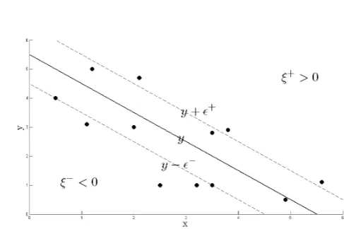
Figure 3: Regression with ǫ-insensitive tube
The regression SVM will use a more sophisticated penalty function than be-fore, not allocating a penalty if the predicted valueyi is less than a distance
ǫaway from the actual value ti, i.e. if |ti−yi|< ǫ. Referring to Figure 3,
the region bound byyi±ǫ∀i is called anǫ-insensitive tube. The other
mod-ification to the penalty function is that output variables which are outside the tube are given one of two slack variable penalties depending on whether they lie above (ξ+
) or below (ξ−) the tube (whereξ+>
0, ξ− >0∀i):
ti≤yi+ǫ+ξ+ (3.2)
ti≥yi−ǫ−ξ− (3.3)
The error function for SVM regression can then be written as:
C
L
X
i=1
(ξi++ξi−) +1 2kwk
2
(3.4)
This needs to be minimized subject to the constraints ξ+ ≥ 0, ξ− ≥ 0 ∀i
α+i ≥0, α−i ≥0, µ+
setting the derivatives to 0: ∂LP
Substituting (3.6) and (3.7) in, we now need to maximize LD with respect
toα+i and α−i (αi+≥0, αi−≥0 ∀i) where:
Substituting (3.6) into (3.1), new predictionsy′ can be found using:
y′ =
This gives us:
b=ts−ǫ− L
X
m∈=S
(αm+−α−m)xm·xs (3.13)
As before it is better to average over all the indicesiinS:
b= 1 Ns
X
s∈S
"
ts−ǫ− L
X
m∈=S
(αm+−α−m)xm·xs
#
3.2 Application
In order to use an SVM to solve a regression problem we need to:
• Choose how significantly misclassifications should be treated and how large the insensitive loss region should be, by selecting suitable values for the parameters C and ǫ.
• Find α+ and α− so that:
is maximized, subject to the constraints
0≤α+i ≤C, 0≤α−i ≤C and
L
X
i=1
(α+i −α−i ) = 0∀i.
This is done using a QP solver.
• Calculatew=
• Determine the set of Support VectorsS by finding the indicesiwhere 0< α≤C and ξi = 0.
• Each new pointx′ is determined by evaluating
y′ =
L
X
i=1
4
Nonlinear Support Vector Machines
4.1 Theory
When applying our SVM to linearly separable data we have started by creating a matrixH from the dot product of our input variables:
Hij =yiyjk(xi,xj) =xi·xj =xTi xj (4.1)
k(xi,xj) is an example of a family of functions called Kernel Functions (k(xi,xj) = xT
i xj being known as a Linear Kernel). The set of kernel
functions is composed of variants of (4.2) in that they are all based on cal-culating inner products of two vectors. This means that if the functions can be recast into a higher dimensionality space by some potentially non-linear feature mapping function x 7−→ φ(x), only inner products of the mapped inputs in the feature space need be determined without us needing to ex-plicitly calculateφ.
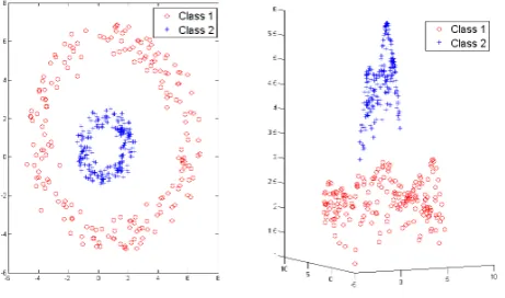
The reason that this Kernel Trick is useful is that there are many classi-fication/regression problems that are not linearly separable/regressable in the space of the inputsx, which might be in a higher dimensionality feature space given a suitable mappingx7−→φ(x).
Figure 4: Dichotomous data re-mapped using Radial Basis Kernel Refering toFigure 4, if we define our kernel to be:
k(xi,xj) =e
− kxi−xjk
2
2σ2
!
feature space (right hand side of Figure 4) defined implicitly by this non-linear kernel function - known as aRadial Basis Kernel.
Other popular kernels for classification and regression are the Polynomial Kernel
k(xi,xj) = (xi·xj+a)b and theSigmoidal Kernel
k(xi,xj) = tanh(axi·xj−b)
whereaand bare parameters defining the kernel’s behaviour.
4.2 Application
In order to use an SVM to solve a classification or regression problem on data that is not linearly separable, we need to first choose a kernel and rel-evant parameters which you expect might map the non-linearly separable data into a feature space where it is linearly separable. This is more of an art than an exact science and can be achieved empirically - e.g. by trial and error. Sensible kernels to start with are the Radial Basis, Polynomial and Sigmoidal kernels.
The first step, therefore, consists of choosing our kernel and hence the map-pingx7−→φ(x).
For classification, we would then need to: • CreateH, whereHij =yiyjφ(xi)·φ(xj).
• Choose how significantly misclassifications should be treated, by se-lecting a suitable value for the parameterC.
• Find αso that
is maximized, subject to the constraints
0≤αi≤ C ∀i and L
X
i=1
αiyi = 0.
This is done using a QP solver. • Calculatew=
L
X
i=1
αiyiφ(xi).
• Determine the set of Support Vectors S by finding the indices such that 0< αi≤C. For regression, we would then need to:
• Find α+ and α− so that:
is maximized, subject to the constraints
0≤α+i ≤C, 0≤α−i ≤C and
L
X
i=1
(α+i −α−i ) = 0∀i.
This is done using a QP solver.
• Calculatew=
L
X
i=1
(α+i −α−i )φ(xi).
• Determine the set of Support VectorsS by finding the indicesiwhere 0< α≤C and ξi = 0.
• Each new pointx′ is determined by evaluating
y′ =
L
X
i=1
References
[1] C. Cortes, V. Vapnik, inMachine Learning, pp. 273–297 (1995).
[2] N. Cristianini, J. Shawe-Taylor, An introduction to support Vector Ma-chines: and other kernel-based learning methods. Cambridge University Press, New York, NY, USA (2000).
[3] J. Shawe-Taylor, N. Cristianini, Kernel Methods for Pattern Analysis. Cambridge University Press, New York, NY, USA (2004).
[4] C. J. C. Burges,Data Mining and Knowledge Discovery2, 121 (1998). [5] C. M. Bishop,Pattern Recognition and Machine Learning (Information