modul 8 classification data mining

(1)

Handaru Jati, Ph.D

Universitas Negeri Yogyakarta

handaru@uny.ac.id

Classification

(also known as classification trees or decision trees) is a data mining algorithm

that creates a step-by-step guide for how to determine the output of a new data instance. The

tree it creates is exactly that: a tree whereby each node in the tree represents a spot where a

decision must be made based on the input, and you move to the next node and the next until

you reach a leaf that tells you the predicted output. Sounds confusing, but it's really quite

straightforward. Let's look at an example.

Listing 1. Simple classification tree

[ Will

You Read This

Section? ] /

\

Ye s

No

/ \

[Will You Understand It?]

[Won't Learn It] / \

Yes No

/ \

[Will Learn It] [Won't Learn It]

(2)

instance, and you are able to predict whether this unknown data instance will learn

classification trees by asking them only two simple questions. That's seemingly the big

advantage of a classification tree — it doesn't require a lot of information about the data to

create a tree that could be very accurate and very informative.

One important concept of the classification tree is similar to what we saw in the regression

model from

Part 1

: the concept of using a "training set" to produce the model. This takes a

data set with known output values and uses this data set to build our model. Then, whenever

we have a new data point, with an unknown output value, we put it through the model and

produce our expected output. This is all the same as we saw in the regression model.

However, this type of model takes it one step further, and it is common practice to take an

entire training set and divide it into two parts: take about 60-80 percent of the data and put it

into our training set, which we will use to create the model; then take the remaining data and

put it into a test set, which we'll use immediately after creating the model to test the accuracy

of our model.

Why is this extra step important in this model? The problem is called

overfitting:

If we

supply

too much

data into our model creation, the model will actually be created perfectly,

but just for that data. Remember: We want to use the model to predict future unknowns; we

don't want the model to perfectly predict values we already know. This is why we create a test

set. After we create the model, we check to ensure that the accuracy of the model we built

doesn't decrease with the test set. This ensures that our model will accurately predict future

unknown values. We'll see this in action using WEKA.

This brings up another one of the important concepts of classification trees: the notion of

pruning.

Pruning,

like the name implies, involves removing branches of the classification

tree. Why would someone want to remove information from the tree? Again, this is due to the

concept of overfitting. As the data set grows larger and the number of attributes grows larger,

we can create trees that become increasingly complex. Theoretically, there could be a tree

with

leaves = (rows * attributes)

. But what good would that do? That won't help us at

all in predicting future unknowns, since it's perfectly suited only for our existing training

data. We want to create a balance. We want our tree to be as simple as possible, with as few

nodes and leaves as possible. But we also want it to be as accurate as possible. This is a

trade-off, which we will see.

Finally, the last point I want to raise about classification before using WEKA is that of false

positive and false negative. Basically, a false positive is a data instance where the model

we've created predicts it should be positive, but instead, the actual value is negative.

Conversely, a false negative is a data instance where the model predicts it should be negative,

but the actual value is positive.

(3)

percentage. On the other hand, if you are simply mining some made-up data in an article

about data mining, your acceptable error percentage can be much higher. To take this even

one step further, you need to decide what percent of false negative vs. false positive is

acceptable. The example that immediately comes to mind is a spam model: A false positive (a

real e-mail that gets labeled as spam) is probably much more damaging than a false negative

(a spam message getting labeled as not spam). In an example like this, you may judge a

minimum of 100:1 false negative:positive ratio to be acceptable.

OK — enough about the background and technical mumbo jumbo of the classification trees.

Let's get some real data and take it through its paces with WEKA.

WEKA data set

The data set we'll use for our classification example will focus on our fictional BMW

dealership. The dealership is starting a promotional campaign, whereby it is trying to push a

two-year extended warranty to its past customers. The dealership has done this before and has

gathered 4,500 data points from past sales of extended warranties. The attributes in the data

set are:



Income bracket [0=$0-$30k, 1=$31k-$40k, 2=$41k-$60k, 3=$61k-$75k,

4=$76k-$100k, 5=$101k-$150k, 6=$151k-$500k, 7=$501k+]



Year/month first BMW bought



Year/month most recent BMW bought



Whether they responded to the extended warranty offer in the past

Let's take a look at the Attribute-Relation File Format (ARFF) we'll use in this example.

Listing 2. Classification WEKA data

@attribute IncomeBracket {0,1,2,3,4,5,6,7} @attribute FirstPurchase numeric

@attribute LastPurchase numeric @attribute responded {1,0}

@data

4,200210,200601,0 5,200301,200601,1 ...

Classification in WEKA

(4)

[image:4.595.75.507.208.540.2]

dealership has in its records. We need to divide up our records so some data instances are

used to create the model, and some are used to test the model to ensure that we didn't overfit

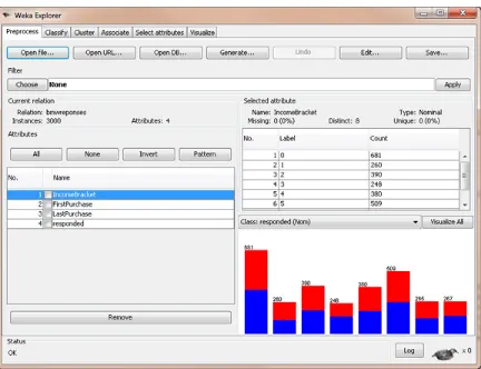
it. Your screen should look like Figure 1 after loading the data.

Figure 1. BMW classification data in WEKA

Like we did with the regression model in

Part 1

, we select the

Classify

tab, then we select the

trees

node, then the

J48

leaf (I don't know why this is the official name, but go with it).

(5)

At this point, we are ready to create our model in WEKA. Ensure that

Use training set

is

selected so we use the data set we just loaded to create our model. Click

Start

and let WEKA

run. The output from this model should look like the results in Listing 3.

Listing 3. Output from WEKA's classification model

Number of Leaves : 28

Size of the tree : 43

Time taken to build model: 0.18 seconds

=== Evaluation on training set === === Summary ===

Correctly Classified Instances 1774 59.1333 % Incorrectly Classified Instances 1226 40.8667 % Kappa statistic 0.1807

(6)

Relative absolute error 95.4768 % Root relative squared error 97.7122 % Total Number of Instances 3000

=== Detailed Accuracy By Class ===

TP Rate FP Rate Precision Recall F-Measure ROC Area Class

0.662 0.481 0.587 0.662 0.622 0.616 1

0.519 0.338 0.597 0.519 0.555 0.616 0

Weighted Avg. 0.591 0.411 0.592 0.591 0.589 0.616

=== Confusion Matrix ===

[image:6.595.70.526.32.339.2]

a b <-- classified as 1009 516 | a = 1

710 765 | b = 0

What do all these numbers mean? How do we know if this is a good model? Where is this

so-called "tree" I'm supposed to be looking for? All good questions. Let's answer them one at a

time:



What do all these numbers mean?

The important numbers to focus on here are the

numbers next to the "Correctly Classified Instances" (59.1 percent) and the

"Incorrectly Classified Instances" (40.9 percent). Other important numbers are in the

"ROC Area" column, in the first row (the 0.616); I'll explain this number later, but

keep it in mind. Finally, in the "Confusion Matrix," it shows you the number of false

positives and false negatives. The false positives are 516, and the false negatives are

710 in this matrix.



How do we know if this is a good model?

Well, based on our accuracy rate of only

59.1 percent, I'd have to say that upon initial analysis, this is not a very good model.



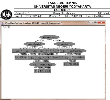
Where is this so-called tree?

You can see the tree by right-clicking on the model you

just created, in the result list. On the pop-up menu, select

Visualize tree

. You'll see

the classification tree we just created, although in this example, the visual tree doesn't

offer much help. Our tree is pictured in Figure 3. The other way to see the tree is to

look higher in the Classifier Output, where the text output shows the entire tree, with

nodes and leaves.

(7)

[image:7.595.72.522.32.442.2]

There's one final step to validating our classification tree, which is to run our test set through

the model and ensure that accuracy of the model when evaluating the test set isn't too

different from the training set. To do this, in

Test options

, select the

Supplied test set

radio

button and click

Set

. Choose the file bmw-test.arff, which contains 1,500 records that were

not in the training set we used to create the model. When we click

Start

this time, WEKA

will run this test data set through the model we already created and let us know how the

model did. Let's do that, by clicking

Start

. Below is the output.

(8)

Comparing the "Correctly Classified Instances" from this test set (55.7 percent) with the

"Correctly Classified Instances" from the training set (59.1 percent), we see that the accuracy

of the model is pretty close, which indicates that the model will not break down with

unknown data, or when future data is applied to it.

However, because the accuracy of the model is so bad, only classifying 60 perent of the data

records correctly, we could take a step back and say, "Wow. This model isn't very good at all.

It's barely above 50 percent, which I could get just by randomly guessing values." That's

entirely true. That takes us to an important point that I wanted to secretly and slyly get across

to everyone: Sometimes applying a data mining algorithm to your data will produce a bad

model. This is especially true here, and it was on purpose.

I wanted to take you through the steps to producing a classification tree model with data that

seems to be ideal for a classification model. Yet, the results we get from WEKA indicate that

we were wrong. A classification tree is

not

the model we should have chosen here. The model

we created tells us absolutely nothing, and if we used it, we might make bad decisions and

waste money.

(9)

but will create a model that's over 88 percent accurate. It aims to drive home the point that

you have to choose the right model for the right data to get good, meaningful information.

modul 8 classification data mining

Handaru Jati, Ph.D

decision must be made based on the input, and you move to the next node and the next until

instance, and you are able to predict whether this unknown data instance will learn

model from

produce our expected output. This is all the same as we saw in the regression model.

of our model.

don't want the model to perfectly predict values we already know. This is why we create a test

pruning.

we can create trees that become increasingly complex. Theoretically, there could be a tree

trade-off, which we will see.

but the actual value is positive.

real e-mail that gets labeled as spam) is probably much more damaging than a false negative

WEKA data set

set are:

Listing 2. Classification WEKA data

it. Your screen should look like Figure 1 after loading the data.

Use training set

What do all these numbers mean? How do we know if this is a good model? Where is this

"Incorrectly Classified Instances" (40.9 percent). Other important numbers are in the

Well, based on our accuracy rate of only

Visualize tree

nodes and leaves.

, select the

will run this test data set through the model we already created and let us know how the

unknown data, or when future data is applied to it.

to everyone: Sometimes applying a data mining algorithm to your data will produce a bad

the model we should have chosen here. The model

Further reading