AUTOMATIC INDOOR BUILDING RECONSTRUCTION FROM MOBILE LASER
SCANNING DATA
Lei Xiea, Ruisheng Wanga,∗
a
Department of Geomatics Engineering, University of Calgary, Calgary, Alberta, T2N 1N4, Canada - (lei.xie, ruiswang)@ucalgary.ca
KEY WORDS:Mobile LiDAR, Point Clouds, Indoor Building Reconstruction, Graph Cut Based Optimization, Door Detection, Room Segmentation
ABSTRACT:
Indoor reconstruction from point clouds is a hot topic in photogrammetry, computer vision and computer graphics. Reconstructing indoor scene from point clouds is challenging due to complex room floorplan and line-of-sight occlusions. Most of existing methods deal with stationary terrestrial laser scanning point clouds or RGB-D point clouds. In this paper, we propose an automatic method for reconstructing indoor 3D building models from mobile laser scanning point clouds. The method includes 2D floorplan generation, 3D building modeling, door detection and room segmentation. The main idea behind our approach is to separate wall structure into two different types as the inner wall and the outer wall based on the observation of point distribution. Then we utilize a graph cut based optimization method to solve the labeling problem and generate the 2D floorplan based on the optimization result. Subsequently, we leverage anα-shape based method to detect the doors on the 2D projected point clouds and utilize the floorplan to segment the individual room. The experiments show that this door detection method can achieve a recognition rate at 97% and the room segmentation method can attain the correct segmentation results. We also evaluate the reconstruction accuracy on the synthetic data, which indicates the accuracy of our method is comparable to the state-of-the art.
1. INTRODUCTION
Recent years have witnessed an increasing demand for highly ac-curate and fidelity indoor 3D models in the areas of indoor map-ping and navigation, building management, virtual reality, and more (Schnabel et al., 2007). Meanwhile, with the decreasing price of laser scanner, it is easier to gain point clouds data from the consumer-level laser scanners (e.g., Hokuyo, RPLiDAR) (Hum-mel et al., 2011). Current methods in 3D indoor building recon-struction is either a manual or interactive tedious process which is time-consuming and error-prone (Tang et al., 2010). Compared to the outdoor reconstruction, the reconstruction of architectural elements is still in early stage, but draws increased attention from the communities like photogrammetry, computer vision and com-puter graphics.
In order to increase the efficiency of indoor building models gen-eration, we propose an automatic reconstruction method based on the observation of the specific distributions of indoor point clouds. The proposed method includes 2D floorplan extraction, door detection, room segmentation and 3D building modeling. We leverage the data from both mobile laser scanner and syn-thetic point clouds to verify the effectiveness of our method.
2. RELATED WORKS
Several efforts have been made on 3D indoor reconstruction from LiDAR data in recent years. We group the existing methods in terms of data acquisition methods: indoor mobile laser scanning and stationary terrestrial laser scanning.
2.1 Indoor Mobile Laser Scanning
(Sanchez and Zakhor, 2012) introduce an approach that divides indoor points into ceilings, floors, walls and other small architec-tural structures according to the normals computed from the PCA
∗Corresponding author
(principle component analysis). Then the RANSAC plane fitting is employed to detect planar primitives for 3D model genera-tion. (Xiao and Furukawa, 2014) generate 2D CSG (Constructive Solid Geometry) models then stack over these models through a greedy algorithm to create 3D CSG models. During the process-ing of the 2D CSG models, they need to compute a free space score of the objective function, requiring the line-of-sight infor-mation from each point to the laser scanner. (Turner and Zakhor, 2014) (Turner et al., 2015) use a back-pack system consisting of a laser scanner, IMU and computer to acquire indoor point clouds while walking around a building. They employ Delaunay trian-gulation to label different rooms. However, their approach needs the number of rooms as a prior knowledge for the seed triangles. Also, their approach requires the timestamp information to re-cover the line-of-sight information from each point to the laser scanner for computing the label scores. (Nakagawa et al., 2015) employ a point-based rendering method to generate range images from point clouds. The detected boundaries in these range images are traced back to point clouds to generate 3D polygons.
2.2 Stationary Terrestrial Laser Scanning
Input Point clouds Preprocessing Floorplan Extraction Door Detection Room Segmentation Output Model
Figure 1. The Pipeline of Methodology: 1) preprocessing; 2) floorplan extraction; 3) door detection; 4) room segmentation; 5) output 3D modeling.
clouds into several planar surfaces such as walls, roofs and ceil-ings, but their method just focuses on the single room reconstruc-tion. (Ikehata et al., 2015) introduce a new framework that de-fines a structure graph and grammar for an indoor scene geom-etry, which can be extended to add additional details. However, their method is based on the Manhattan world assumption that restricts the types of geometric expressions. Another approach proposed by (Mura et al., 2014) explores the vertical structure (i.e. planar patches from the walls) and a visibility check to elim-inate occlusions through the position of static laser scanner. The main limitation is that their method can’t deal with data contain-ing rooms with different heights. (Thomson and Boehm, 2015) introduce a concept of Industry Foundation Classes (IFC), a term from BIM. They use IFC to describe the building structure and a RANSAC-based method for planar model generation.
As we can see, most of existing methods need to know the line-of-sight information from each point to the laser scanner. In this paper, we propose a pipeline that works for data without the line-of-sight information.
3. METHODOLOGY
Figure 1 illustrates the pipeline of our method containing five parts. The first step is the preprocessing to remove noises. Sec-ondly, we use a graph-cut based algorithm to extract the floorplan on 2D projected points. The third and fourth steps are door de-tection and room segmentation, respectively. Finally, we utilize information from floorplan, door positions and room segmenta-tion results to generate the 3D building models. The input data consists of two parts: raw point clouds (x-y-z coordinates with in-tensity values) and trajectory of mobile laser scanner (we convert it into discrete points by 1 meter interval).
3.1 Preprocessing
Figure 2a shows the point clouds containing various noises, es-pecially near the windows and doors. This is a consequence of laser beams which traverse the transparent material or go across the opening doors. These beams will strike the objects outside of the building and generate isolated points outside of the building. The points near the window and other highly transparent mate-rials have a relatively low echo intensity value. For this reason, we can set a threshold to remove the points whose intensity is below the threshold. Similar to the (Ikehata et al., 2015), we set a thresholdIth = µi−α·δi, where theµiandδidenotes the mean value and standard deviation of intensity. Then we utilize the morphological operations (i.e., opening operation, the largest connected component) to eliminate isolated points that cannot be removed by intensity threshold. The Figure 2b shows the results of preprocessing.
3.2 Floorplan Extraction
The floorplan extraction contains two steps: 1) linear primitive extraction, 2) cell selection.
(a) (b)
Figure 2. a) The original data and close-up views showing the noisy points penetrating windows or passing through open
doors; b) The result after the preprocessing step.
3.2.1 Linear Primitive Extraction Rather than a Manhattan structure, we only assume that the walls are perpendicular to the floor. In other words, walls don’t need to be perpendicular to each other. To obtain the vertical structure, we use the PCA (prin-ciple component analysis) to estimate the normal for each point and flip the normal direction if it isn’t towards the nearest scan-ner position. If
is smaller than a threshold (i.e. 0.01),
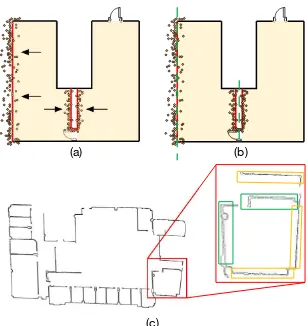
we consider the point belonging to the wall, andNz here is the unit vector of the Z axis. We then project the walls to the x-y plane and apply a RANSAC line fitting algorithm to fit the lin-ear primitives. The RANSAC algorithm will discard the lines which contain points less than a threshold (i.e. 15). Similar to the approaches (Ikehata et al., 2015) and (Michailidis and Pajarola, 2016), we extract the representative lines of the candidate walls using a 1D mean shift clustering. The first step is to perform the clustering according to the orientations of the walls, then compute the most likely offset for each line. The candidate walls (repre-sentative lines) are generated at the peaks of the offsets as shown in Figure 3.
(a) (b)
Figure 3. a) The linear primitives from RANSAC line fitting; b) The result from the line clustering.
3.2.2 Cell Selection To generate floorplan, we need to use the linear primitives from previous step to define the outline for each room. The idea is to convert the line segments into cells. We check the intersections of different lines and then partition the ground plan into several cells. After the cell decomposition, we can obtain a set of cellsT ={Ti
i= 1, ..., n}as shown in
extract the outer walls by the adjacent edges with different labels from the cells. As shown in Figure 4b, we use this global min-imization method to label the different cells to the exterior cells (yellow) and interior cells (green). The details of the processing are in the following.
(a) (b)
(c) (d)
Figure 4. Floorplan extraction: a) cell decomposition; b) room labeling; c) outer wall extraction; d) inner wall extraction.
Graph generation: An undirected graph G =< V,E >can be defined to encode the set of cells T to the label setL =
{Lint,Lext}. The cells setT can be assigned to the vertices in the graph. Each edge in the graph is assigned with a non-negative weightwe. The set of edgeEis composed of two parts: n-links (neighborhood links) and t-links (terminal links). Therefore, the set of edgeEcan be expressed asE =
{v, S},{v, T}
S
N . TheN represents the links of neighborhood. The sets
SandT denote the “source” and “sink” nodes representing fore-ground and backfore-ground in graph cut algorithm, respectively. More specifically, the source node is labelled as interior spaceLint, and the sink node is exterior spaceLext. The energy function can be represented as
where the first termDi(Li) is the data term, representing the penalty of assigning every vertex to different labels; the second termSi,j(Li, Lj)is smoothness term multiplying with an indica-tor functionδ(Li 6=Lj)which is the pairwise cost for adjacent cells to ensure the smoothness of segmentation. The parameterλ
is used to define the importance of the data term versus smooth-ness term.
Smoothness Term: A weightwi,j is defined to determine the weight between adjacent cells, denoting the shared edges between the connected cells. The weightwi,jcan be computed through a grid map derived from the horizontal bounding box of the lin-ear primitives. As shown in Figure 5, we can divide the walls into two categories as inner walls and outer walls. The outer wall separating the indoor and outdoor scenes will be just scanned on single side. However, the inner wall will be scanned on both sides which results in an empty region between two sides of the wall. The green dashed lines in Figure 5b denote the representa-tive lines from RANSAC line fitting and clustering. For the outer walls, the extracted lines are normally close to the wall. How-ever, for the inner walls, the extracted lines are often located in the middle of the wall. The Figure 5c shows an example from our data. The walls in the green rectangles are inner walls scanned on both sides and the walls in the yellow rectangles are outer walls scanned only on single side. Therefore, there exists empty areas within the inner walls.
(a) (b)
(c)
Figure 5. The illustration of points distributions. a), b) Scanning process: the black arrows indicate the directions of the scanning, showing different point distributions on outer and inner walls. c)
The points distributions on the real data, inner walls (green rectangles) and outer walls (yellow rectangles)
We calculate two weights for each line taking outer and inner walls into account. Figure 6 indicates two different patterns of the weight definition and the grey dashed lines indicate the cells from the cell decomposition. We generate both 1-column grid map and 3-column grid map centered at the edge of the cell, and compute the weight as the ratio of occupied grids. Therefore, the weights can be calculated using the following equation,wi,j,k=
occ(ei,j)
sum(ei,j), where the weightwi,j,k is the weight on each edge, occ(ei,j) andsum(ei,j)represent the number of occupied grids
and the total number of grids, respectively. Theei,jrepresents the edge between different cells,i,jis the index of cells andkis the column number of grid map. The final weight for each edge is selected using the following equation:
wi,j=
(
wi,j,3, wi,j,3−wi,j,1≥H wi,j,1, otherwise
(2)
whereHis an experimentally chosen constant (i.e. 0.3). And the smoothness term can be determined as
Si,j(Li, Lj) = 1−wi,j (3)
Note that we also usewi,jas a prior knowledge for wall identifi-cation to determine data term in the following step.
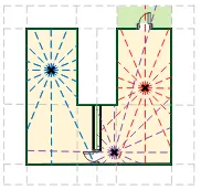
Data Term:Inspired by the method (Ochmann et al., 2014), we use a ray casting method to evaluate the weight between the cells and the terminal nodes. Since we don’t have the line-of-sight in-formation from the laser scanner to the point, we cannot use the ray information directly. Instead, we propose a new method to define the data term by creating virtual rays based on the scanner positions from the trajectory for estimating the likelihood of dif-ferent labels. The rationale is that the cells belonging to interior space will be intersected by the rays more than the exterior ones. In Figure 7, the black crosses are the positions of the scanner, and the dashed lines launched from the crosses are the simulated rays. If the rays intersect with the walls (the green lines), we count it to the weight for the data term. Naturally, the outer cells (green and white background cells) will have relatively low weights and the interior cells will have relatively high weights (yellow back-ground cells).
(a) (b)
Figure 6. Different patterns of the weight definition. The dashed grey lines depict the result of the cell decomposition. a) 1
column grid map; b) 3 columns grid map.
at the device location. If the weight of an edgewi,j is greater than a threshold (i.e. 0.55), we consider the edge as a wall. For the sake of eliminating the bias of different sizes of cells, the data term is scaled by an area scalable parametersα. The data term can be represented by the following function:
Di(Li) =
(
(1− inum
maxnum)·sα, Li∈ext
inum
maxnum ·sα, Li∈int
(4)
whereinumis the intersection number of each cell,maxnumis the maximum number of each cell,sαthe reciprocal of each cell’s area.
Once the cells are labelled as exterior or interior cells, we can ex-tract the outer walls from the adjacent edge between two different labels as shown in Figure 4c (the red lines). The weight definition of the inner walls are different from the outer walls’. As discussed before, if the weight of cell sufficeswi,j =wi,j,3−wi,j,1≥0.3,
we consider it as an inner wall as shown in Figure 4d (the cadet blue lines). Both the outer and inner walls together constitute the floorplan.
Figure 7. Simulated ray casting from the scanner positions. The yellow cells present a high likelihood of being interior cells, and
the green and white cells are likely to be the exterior cells.
3.3 Door detection
We use a reasonable assumption that the doors are opened during the data acquisition process as the mobile laser scanner needs to enter and exit the rooms. Under this assumption, we can con-vert the door detection problem to find the vacancy in the point clouds. We propose a new method based on the properties of the Delaunay triangulation, alpha-shape and the scanner trajectory in the projected 2D space.
The alpha-shape algorithm (Edelsbrunner et al., 1983) has been widely used in determining the boundaries of the points clouds especially of outdoor buildings (Wei, 2008)(Albers et al., 2016). In the actual implemtation, alpha algorithm is starting from a De-launay triangulation and selecting boundaries in the DeDe-launay tri-angles. An alpha value(0< α <∞) is a parameter imposing the precision of final boundary. A large value (α→ ∞) results in the alpha boundary of a convex hull while a small value (α→0) means that every point can be the boundary point. As shown in the Figure 8a, the green circles indicate the gaps from the doors and the yellow circles show the gaps from the occlusions.
(a)
(b) (c) (d)
Figure 8. Top: the gaps in 2D point projection, the green circles represent the gap deriving from the real door while the gaps in the yellow circles resulting from occlusions. Bottom: three steps
of door detection.
We can see that the doors’ widths are relatively wider than those of the occlusions. Also the gaps from the doors are shorter than the hallway or other structures such as an extrusion along the hall way. Therefore, the sizes of the door gaps are significantly differ-ent from any other structures or occlusions in the indoor scene. We can assume that different values of the alpha parameters will lead to the differences of the alpha interior triangles. A portion of the triangles can represent the doors, and the set of the different triangles can be represented as
Tdif f=Thigh− Tlow (5)
In this equation,Thighis a set of interior triangles from a high alpha value, andTlowis a set of interior triangles from a low alpha value. We set alpha values asαhigh = 0.88andαlow = 0.78. The set of green trianglesTdif f as shown in Figure 8b contains the doors. The green triangles near the outer walls intersected by the trajectory of the laser scanner or the simulated rays will be considered as the door candidates (the blue triangles in Figure 8c). In order to alleviate some bias, we set a threshold of the intersection number as 10 and discard the candidate doors less than a certain threshold (i.e., 0.6m). Finally, we can use blue triangles to produce the floorplan with door representations as shown in Figure 8d.
3.4 Room Segmentation
Li,j =
(
Li=Lj, (ci, cjare adjacent) T(Eijis not wall)
Li6=Lj, otherwise
(6) whereEijdenotes the shared edge between two adjacent cells, the property of each edge can be gained from extracted floorplan. We randomly select some cells as seed points and label cells iter-atively according to the above metrics. Figure 9 shows the results of room segmentation, the segmented regions including rooms and corridors. The indoor scenes have been separated into 9 re-gions and 18 rere-gions on the 2D floorplan, respectively.
(a) (b)
Figure 9. Results of room segmentation (including rooms and corridors): a) office 1 with 9 regions; b) office 2 with 18 regions.
Utilizing the result of room segmentation as a boundary of every room, we employ the elevation histograms to estimate the heights of rooms. Finally, we stretch up the walls for the 3D model gen-eration.
4. EXPERIMENT
The proposed method is evaluated on two point cloud datasets and one synthetic point clouds. The experiments are running on a computer with an Inter i7-4770 CPU @ 3.4GHz and 10.0 GB ram. We implement this method based on the open source libraries: Point Cloud Library (PCL), Computational Geometry Algorithms Library (CGAL) and Mobile Robot Programming Toolkit (MRPT) for our system.
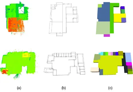
Figure 10 shows the reconstruction results from two mobile laser scanning point clouds. Figure 10a is the original point clouds and Figure 10b is the wireframe models without ceilings in which we can observe the structures of doors and walls clearly, Figure 10c is the 3D reconstructing result. Table 1 shows that all the rooms are successfully reconstructed and all the doors except one door are detected. The missing door is because the door was closed during the data acquisition, which conflict with our assumption that all the doors are opened.
Input Office 1 Office 2 Synthesis
# of points [million] 23.3 52.2 0.8
# of rooms 9 18 3
# of doors 13 22 4
Output Office 1 Office 2 Synthesis
# of rooms 9 18 3
# of doors 12 22 4
Table 1. Description of the input data and statistics of the outputs
In order to evaluate the accuracy of the proposed method, a set of synthetic point clouds is employed. We create a Sketchup model and sample it to point clouds by Meshlab. The synthetic data is
(a) (b) (c)
Figure 10. Experiment results. From left to right: the original point clouds, wireframe models without ceilings, reconstruction
models with ceilings.
(a) (b) (c)
Figure 11. Accuracy evaluation: a) point clouds with
σ= 10mmGaussian noise; b) wireframe model; c) quantitative evaluation of the reconstructed surfaces and supporting points.
added with 10% Gaussian noises as shown in the left of Figure 11. The reconstruction errors are measured by the distances from points to the corresponding reconstructed surfaces. The right of Figure 11 shows the color maps of the reconstruction errors. The maximum fitting error, minimum fitting error and the average fit-ting error turned out to be 2.52cm, 0.58cm, 1.77cm, respectively.
5. CONCLUSIONS
We propose a complete methodology for indoor building recon-struction from mobile laser scanning data. Our system can gen-erate floorplan, detect doors, segment each individual rooms, and 3D indoor modeling. Different from existing methods, our method doesn’t need line-of-sight information and can deal with both outer and inner wall detection. The experiments on the real point clouds and synthetic point clouds demonstrate the effectiveness and high accuracy of our method. The limitations of our method that it will fail if the indoor scene contains cylindrical or spherical walls, sloping walls and it will discard some details in the global optimization.
For the future work, we plan to reconstruct more detailed indoor scene by extending our method in a 3D view and employ im-ages acquired simultaneously with the point clouds to enhance the modeling performance.
REFERENCES
Albers, B., Kada, M. and Wichmann, A., 2016. Automatic extrac-tion and regularizaextrac-tion of building outlines from airborne lidar point clouds.ISPRS-International Archives of the
Photogramme-try, Remote Sensing and Spatial Information Sciencespp. 555–
Boykov, Y. Y. and Jolly, M.-P., 2001. Interactive graph cuts for optimal boundary & region segmentation of objects in nd images.
In: Computer Vision, 2001. ICCV 2001. Proceedings. Eighth
IEEE International Conference on, Vol. 1, IEEE, pp. 105–112.
Budroni, A. and B¨ohm, J., 2010. Automatic 3d modelling of indoor manhattan-world scenes from laser data. In:ISPRS Symp.
Close Range Image Measurement Techniques, Vol. 2.
Edelsbrunner, H., Kirkpatrick, D. and Seidel, R., 1983. On the shape of a set of points in the plane.IEEE Transactions on
infor-mation theory29(4), pp. 551–559.
Hummel, S., Hudak, A., Uebler, E., Falkowski, M. and Megown, K., 2011. A comparison of accuracy and cost of lidar versus stand exam data for landscape management on the malheur national forest.Journal of forestry109(5), pp. 267–273.
Ikehata, S., Yang, H. and Furukawa, Y., 2015. Structured indoor modeling. In:Proceedings of the IEEE International Conference
on Computer Vision, pp. 1323–1331.
Michailidis, G.-T. and Pajarola, R., 2016. Bayesian graph-cut optimization for wall surfaces reconstruction in indoor environ-ments.The Visual Computerpp. 1–9.
Mura, C., Mattausch, O., Villanueva, A. J., Gobbetti, E. and Pa-jarola, R., 2014. Automatic room detection and reconstruction in cluttered indoor environments with complex room layouts.
Com-puters & Graphics44, pp. 20–32.
Nakagawa, M., Yamamoto, T., Tanaka, S., Shiozaki, M. and Ohhashi, T., 2015. Topological 3d modeling using indoor mo-bile lidar data. The International Archives of Photogrammetry,
Remote Sensing and Spatial Information Sciences40(4), pp. 13.
Ochmann, S., Vock, R., Wessel, R., Tamke, M. and Klein, R., 2014. Automatic generation of structural building descriptions from 3d point cloud scans. In:Computer Graphics Theory and
Applications (GRAPP), 2014 International Conference on, IEEE,
pp. 1–8.
Oesau, S., Lafarge, F. and Alliez, P., 2014. Indoor scene recon-struction using feature sensitive primitive extraction and
graph-cut. ISPRS Journal of Photogrammetry and Remote Sensing90,
pp. 68–82.
Previtali, M., Barazzetti, L., Brumana, R. and Scaioni, M., 2014. Towards automatic indoor reconstruction of cluttered building rooms from point clouds.ISPRS Annals of the Photogrammetry,
Remote Sensing and Spatial Information Sciences2(5), pp. 281.
Sanchez, V. and Zakhor, A., 2012. Planar 3d modeling of building interiors from point cloud data. In: Image Processing (ICIP),
2012 19th IEEE International Conference on, IEEE, pp. 1777–
1780.
Schnabel, R., Wahl, R. and Klein, R., 2007. Efficient ransac for point-cloud shape detection. In: Computer graphics forum, Vol. 26number 2, Wiley Online Library, pp. 214–226.
Tang, P., Huber, D., Akinci, B., Lipman, R. and Lytle, A., 2010. Automatic reconstruction of as-built building information models from laser-scanned point clouds: A review of related techniques.
Automation in construction19(7), pp. 829–843.
Thomson, C. and Boehm, J., 2015. Automatic geometry genera-tion from point clouds for bim.Remote Sensing7(9), pp. 11753– 11775.
Turner, E. and Zakhor, A., 2014. Floor plan generation and room labeling of indoor environments from laser range data. In: Com-puter Graphics Theory and Applications (GRAPP), 2014
Inter-national Conference on, IEEE, pp. 1–12.
Turner, E., Cheng, P. and Zakhor, A., 2015. Fast, automated, scalable generation of textured 3d models of indoor environ-ments. IEEE Journal of Selected Topics in Signal Processing 9(3), pp. 409–421.
Wei, S., 2008. Building boundary extraction based on lidar point clouds data.Proceedings of the International Archives of the Pho-togrammetry, Remote Sensing and Spatial Information Sciences 37, pp. 157–161.