ESTIMATING EXTERIOR ORIENTATION PARAMETERS OF HYPERSPECTRAL
BANDS BASED ON POLYNOMIAL MODELS
A. Berveglieri a, *, A. M. G. Tommaselli a, E. Honkavaara b
a UNESP, São Paulo State University, Dept. of Cartography, 19060-900 Presidente Prudente – São Paulo, Brazil –
[email protected], [email protected]
b Finnish Geospatial Research Institute FGI, Kirkkonummi, Finland – [email protected]
Commission ΙΙI, WG III/4
KEY WORDS: FPI camera, Image orientation, Photogrammetry, Polynomial model, UAV
ABSTRACT:
Hyperspectral camera operating in sequential acquisition mode produces spectral bands that are not recorded at the same instant, thus having different exterior orientation parameters (EOPs) for each band. The study presents experiments on bundle adjustment with time-dependent polynomial models for band orientation of hyperspectral cubes sequentially collected. The technique was applied to a Rikola camera model. The purpose was to investigate the behaviour of the estimated polynomial parameters and the feasibility of using a minimum of bands to estimate EOPs. Simulated and real data were produced for the analysis of parameters and accuracy in ground points. The tests considered conventional bundle adjustment and the polynomial models. The results showed that both techniques were comparable, indicating that the time-dependent polynomial model can be used to estimate the EOPs of all spectral bands, without requiring a bundle adjustment of each band. The accuracy of the block adjustment was analysed based on the discrepancy obtained from checkpoints. The root mean square error (RMSE) indicated an accuracy of 1 GSD in planimetry and 1.5 GSD in altimetry, when using a minimum of four bands per cube.
* Corresponding author
1. INTRODUCTION
There is a growing interest in the use of high resolution remote sensing using hyperspectral frame cameras, which have been developed recently. The availability of new lightweight sensors (Aasen et al., 2015; Gupta et al., 2008; Hagen and Kudenov, 2013; Lapray et al., 2014) and the improvement of the autonomy of unmanned aerial vehicles (UAVs) have contributed for applications in forestry, agriculture, water and natural resources management (e.g., Goetz, 2009; Honkavaara et al., 2013). Research and monitoring activities have been benefited by the possibility of acquiring images with high spatial, temporal and spectral resolution, which enables more detailed studies based on image analysis.
The Rikola camera model (by Senop Ltd.) is a type of these hyperspectral framing sensors currently available, which can be carried by UAV platforms for remote sensing applications. Its technology is based on a tunable Fabry-Perot Interferometer (FPI) installed inside the optical system and allows capturing cubes of images sequentially. Each image cube is composed of a set of spectral bands that are defined by the air gap values of the FPI, which covers the spectral range from 500 to 900 nm with two sensors. Another technical feature of the FPI camera is that the spectral bands are not recorded at the same instant. The bands are sequentially acquired following a time interval (dependent on the number of bands) set by the manufacturer. Due to the sequential acquisition, the individual bands in each cube have different exterior orientation parameters (EOPs), when collecting images from a moving platform.
Typically for mapping tasks with high spatial resolution, accurate 3D data are required. Thus, EOPs must be determined with high accuracy to describe the position and attitude of the camera. A problem is that UAV platforms can be unstable during the flight due to mechanical vibrations or wind gust, which can affect the planned trajectory. EOPs can be determined directly by a GPS/inertial system, indirectly by bundle block adjustment, or by integrated sensor orientation (ISO), this last being a combination of the two previous techniques.
Because determination of EOPs for each band is labour intensive and time consuming task, this study investigated a time-dependent technique for simultaneous image orientation including all bands of a hypercube. The main objective was to define suitable polynomial models and weights for constraints for EOP estimation of the entire cube using a minimum set of bands. Thus, EOPs of the entire cube can be estimated without requiring a band by band bundle adjustment (BA) with all bands, which would be complicated due to the large number of image cubes (thousands of cubes) that can result from a production aerial survey.
2. FPI FRAMING CAMERA
light rays passing through the FPI undergo multiple reflections. The length of the optical path produces different wavelengths, which are spectral bands generated as a function of the interferometer air gap. With several air gap values, a set of wavelengths varying between 500 nm and 900 nm can be produced using two CMOS sensors redirected by a beam splitting device (Oliveira et al., 2016).
Figure 1. Rikola camera model and a sketch representing its internal system. Source: Oliveira et al. (2016).
Table 1 shows the main features of the Rikola camera used in this study. The hyperspectral images are captured as data cubes with a number of predefined bands. The number of spectral sequential acquisition during the platform displacement. The default mode implemented in the camera only grab the GPS time of the first band in the cube. The positions of the subsequent spectral bands in the cube should be estimated by interpolation using a sequence delay calculator provided by the manufacturer.
Camera model Rikola FPI2015 Nominal focal length 9 mm
Pixel size 5.5 μm
Image dimension 1017 × 648
Sensors CMOS
Spectral resolution 10 nm, FWHM (full width at half maximum)
Weight ~ 700 g
Table 1. Technical features.
Figure 2. Band acquisition in a hyperspectral cube during an aerial survey.
3. MODELLING EOPS WITH POLYNOMIALS
The positions and attitute of the acquisition platform vary as a function of time. Thus, camera EOPs can be estimated by polynomials that model the band displacement and rotations in the cube. A set of second-order polynomials is presented in Eq. (1) to model the position (X, Y, Z) and attitude (ω, φ, κ) of each spectral band in the hypercube as a function of time. The set of polynomials is formed by eighteen parameters that refer to platform speed (ai) and acceleration (bi). The time interval t each band is time consuming. Furthermore, accurate direct orientation with UAVs is a challenging task because of the costs and weight of high-grade inertial navigation systems. In our case, we have assembled a UAV with the hyperspectral camera connected to GPS/IMU (inertial measurement unit) sensors to collect direct georeferencing data. A hardware solution using event logging has been developed on the camera to enable recording of the GPS time of each band. This is possible because the FPI camera sends one pulse per band. Such pulses are received by a dual-frequency GPS/inertial system, and the time of each event is recorded in the raw file for post-processing.
The proposed technique uses polynomial models integrated into the BA. Instead of computing the EOPs of each individual band, the displacements and attitude changes of the hyperspectral bands, with respect to the first one, are modelled by time-dependent polynomial functions. The objective is to estimate the polynomial parameters simultaneously with the BA using few bands and then interpolate the EOPs to the other bands of the cube. The technique is based on the adjustment method combined with weighted constraints on the EOPs and is similar to the technique proposed by Tommaselli and Marcato Junior (2012) for pushbroom satellite image orientation (i.e. linear sensor). However, the technique in this study was adapted to a frame sensor and applied to sequential images in hyperspectral cubes.
4. DATA, EXPERIMENTS AND RESULTS
images were generated to study the effects resulting from the use of polynomial parameters in the BA. Next, the proposed technique was applied to a set of hyperspectral images to assess its potential with real data.
4.1 Simulated data
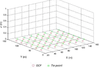
A set of simulated data was generated to analyse the behaviour of the polynomial parameters. Flying height and speed, GSD and image overlap were designed analogously to a hyperspectral aerial survey with UAV. In this configuration, IOPs (focal length = 8 mm and principal point (0, 0)) were considered perfect and without lens distortion effects. Four cubes with 10 bands each one forming a flying strip were simulated. EOPs were determined in a trajectory simulating a sequential acquisition based on nominal camera acquisition interval, with flying height = 160 m, flying speed = 4 m/s, image overlap = 70% and GSD = 10 cm. The image coordinates were disturbed with the addition of Gaussian noise (σ = 0.5 pixel) to introduce random errors. Figure 3 shows the grid of ground points generated in the object space to be used either as tie points or control points, in a local reference system.
Figure 3. Simulated GCPs and tie points for the trials.
4.2 Analysis of the polynomial parameters
Experiments were performed to analyse the behaviour of the results with BAPM (bundle adjustment with polynomial models). Twenty eight GCPs and seventy two tie points were used to estimate the EOPs that were analysed based on seven checkpoints. A configuration for the EOPs was fixed and then different weighted constraints were applied to the polynomial parameters to test the BAPM. The experiments with image orientation to be presented were performed with four bands to estimate the EOPs of the ten band of a sensor. The same experiment was carried out using all ten bands and a similar effect was observed.
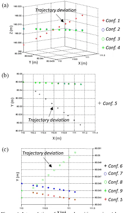
Firstly, the polynomial parameters related to speed in XYZ (ai) were weighted with variations on their standard deviations, while the acceleration parameters (bi = 1.10-11) were kept with absolute constraints, which is equivalent to reduce the polynomial to a straight line model. Table 1 presents how the standard deviations (σ) were considered in the experiments, which were tried in eleven configurations. In all experiments, the BAPM obtained the same accuracy in the checkpoints, which were assessed by the root mean square error (RMSE) (4 cm in planimetry and 14 cm in altimetry).
Figure 4(a) exemplifies the effect in the band positions (XYZ) in a cube when the 10 bands were interpolated with the configurations from 1 to 5 from the 4-band BAPM. The
sequence highlighted in red indicated that a constraint considering σ = 0.1 m/s used in the three parameters (a1, a2, a3) affected the parameter a3 due to a trajectory deviation in Z, as presented in Figure 4(a). However, the effect was controlled when better constraints were applied to a3 (σ = 0.01 to 1.10-11 m/s). Further experiments showed that the parameters a1 and a2 could not be set as free unknowns in the BAPM. A deviation was produced in the trajectory when a value of 0.5 m/s (configuration 5) was used in σa1 and σa2, as seen in Figure 4(b). Figure 4(c) shows the effect from a4, a5 and a6 when different standard deviations were tested. In this case, when a constraint of 0.0001 rad/s (configuration 8) was imposed to the three parameters (angular velocities), a trajectory deviation was caused in the band positions. However, when larger standard deviations were only used in
σa4 and σa5, better results were obtained.
Configuration (m/s) (rad/s)
σa1 σa2 σa3 σa4 σa5 σa6
1 0.1 0.1 0.1 0.1 0.1 0.0001
2 0.1 0.1 0.01 0.1 0.1 0.0001
3 0.1 0.1 0.001 0.1 0.1 0.0001
4 0.1 0.1 1.10-11 0.1 0.1 0.0001
5 0.5 0.5 0.01 0.1 0.1 0.0001
6 0.01 0.01 0.00001 0.1 0.1 0.0001
7 0.01 0.01 0.00001 0.5 0.5 0.0001
8 0.01 0.01 0.00001 0.0001 0.0001 0.0001
9 0.01 0.01 0.00001 0.1 0.1 0.1
10 0.01 0.01 0.00001 0.5 0.5 0.5
(In red) values that caused trajectory deviation
Table 1. Variation in the standard deviations of the polynomial parameters related to speed in the XYZ used as weighted
Figure 4. Interpolation of ten band positions using 4-band BAPM in a cube considering the configurations (Conf..)
presented in Table 1.
It is known that accelerations are correlated with speeds when computing then indirectly. As speeds are expected to be theoretically constant according to the flight plan, accelerations may occur due to slight variations during flight caused by wind conditions and platform movement, but they should be minimal.
An analysis on the indirect estimation of acceleration parameters (bi) was also performed in a way similar to the previously presented for speeds. In this case, the standard deviation of the parameters (σai) were set (σa1 = σa2 0.01 m/s; σa4 = σa5 = 0.01 rad/s; σa3 = 1.10-6 m/s and σa6 = 1.10-6 rad/s) and then some variations in the standard deviations of σbi were introduced to verify the effects of the corresponding constraints on the band positions. Table 2 shows the several standard deviations used in the constraints to bi, which indicated the greatest effect when a value of 0.5 m/s2 (configuration 1) was used for σb1, σb2 and σb3, as depicted in Figure 5(a). The other parameters b4 to b6 were kept with σ = 1.10-6 rad/s2, since changes in these parameters had no effect on perspective centre (PC) coordinates. As can be seen in Table 2, the parameter b3 requires more restrictive constraint (higher weighted constraint, smaller standard deviation).
Configuration (m/s2) (rad/s2)
σb1 σb2 σb3 σb4 σb5 σb6
1 0.5 0.5 0.5 1.10-6 1.10-6 1.10-6
2 0.5 0.5 0.1 1.10-6 1.10-6 1.10-6
3 0.5 0.5 0.01 1.10-6 1.10-6 1.10-6
4 0.5 0.5 0.001 1.10-6 1.10-6 1.10-6
5 0.1 0.1 0.01 1.10-6 1.10-6 1.10-6
6 0.01 0.01 0.01 1.10-6 1.10-6 1.10-6
(In red) values that caused trajectory deviation
Table 2. Variation in the standard deviations of the polynomial parameters related to acceleration used in the weighted
constraints.
Figure 5. Estimation of ten band positions in a cube considering the configurations (Conf.) presented in Tables 2
and 3.
Another test was performed to analyse the behaviour of b4, b5 and b6 parameters after some changes in the weighted constraints. Standard deviations of 1.10-6 m/s2 and 1.10-6 rad/s2 were assigned to σb1-3and σb4-6 respectively, and then σa4, σa5 and σa6 were varied, since ai should be correlated. Table 3 presents the values used in the trials. The effects represented by the blue sequences in Figure 5(b) were results of using less restrictive constraints (configurations 3 and 4) on σa1 and σa2 (σ = 0.1 m/s). The estimation of parameters a4-6 performed well with smaller constraints (higher standard deviations).
Config. (m/s) (rad/s) (m/s2) (rad/s2)
σa1 σa2 σa3 σa4 σa5 σa6 σb1-3 σb4-6
1 0.01 0.01 1.10-6 0.1 0.1 0.0001
2 0.01 0.01 1.10-6 0.1 0.1 0.1
3 0.1 0.1 1.10-6 0.1 0.1 0.1
4 0.1 0.1 0.1 0.1 0.1 0.1
(In red) values that caused trajectory deviation
4.3 Experiments with the number of bands per cube
The number of bands per cube was tested to assess the feasibility of using an optimum number, since hyperspectral aerial surveys can produce a high number of images with thousands of spectral bands. Thus, an experiment with the polynomial models was conducted with the simulated data to compare the accuracy achieved using different number of bands, as presented in Table 4. For the experiments in sections 4.3-4.5, the following settings were used: σ = 10 cm in XYZ, σ the RMSE in the checkpoints to assess the accuracy. As can be seen, the number of bands had an effect on the image orientation accuracy. When all 10 bands were used, the RMSE in planimetry indicated less than 3.1 cm and altimetry around 14 cm, which were the smallest discrepancies.
#bands RMSE_X (m) RMSE_Y (m) RMSE_Z (m)
10 0.017 0.031 0.140
4 0.021 0.048 0.172
3 0.024 0.049 0.183
Table 4. Simulated data: discrepancies in seven check points considering variations of the number of bands and 28 GCPs.
BAPM with 4 and 3 bands generated larger discrepancies. However, when their RMSEs were compared with those produced with 10 bands, the differences were at the most 2 cm in planimetry and 4.5 cm in height. The smallest RMSE differences were obtained when using 4 bands, which can then be recommended for the application of the polynomial technique.
4.4 Variation of the number of GCPs
The number of GCPs in a BA is also important for the quality of the image orientation. Often the availability of GCPs is scarce in survey areas and therefore only a minimum of points should be used. Thus, the objective was to verify the impact of accuracy when using few GCPs. Moreover, fewer points may reduce the workload on GCP measurement tasks.
A test was performed varying from 4 to 5 GCPs and 7 checkpoints. The RMSE values in the object space obtained from the checkpoints were included in Table 5. Small differences were found among the three XYZ coordinates. The largest difference was obtained in Z with a value of 1.2 cm
Table 5. Simulated data: discrepancies in seven checkpoints using 4 bands and 28 GCPs.
4.5 Variation of the IOPs
Some random perturbation were introduced in the interior orientation parameters (IOPs) to simulate the errors in these
parameters and evaluate the impact on the results. An error of 0.5 pixel was added to the focal length, whereas the principal
Table 6. Simulated data: RMSE in seven checkpoints using four bands and 28 GCPs.
4.6 Experiments with real data
Two scenarios were planned to study the technique in real conditions using data provided by direct georeferencing and considering only camera positions collected by single-frequency GPS receiver.
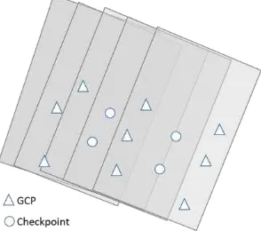
Figure 6. GCPs and checkpoints distributed in the image block.
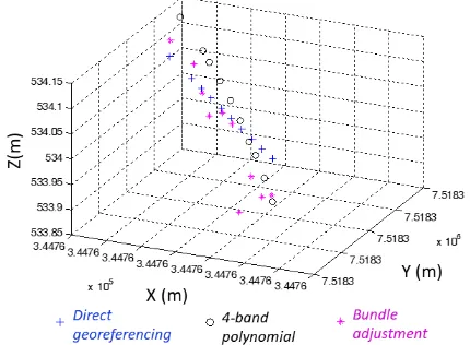
As shown in Table 7, three image orientation procedures using 10 bands of one of the camera sensors were performed for comparison purposes. A conventional BA was run with the 10 bands to be used as reference. The same 10 bands were also estimated by BAPM and a second experiment with BAPM was performed with only 4 bands. The main settings for these procedures were: calibrated IOPs as fixed; camera positions were used as weighted constraints with standard deviation of 20 cm; attitude angles as unknowns; image coordinates with an error of 1 pixel and coordinates of GCPs with standard deviation of 5 cm. Automatic tie points were extracted and used. All procedures were carried out with in-house developed software CMC adapted to perform BAPM.
Technique RMSE_X (m) RMSE_Y (m) RMSE_Z (m)
BA (10 bands) 0.068 0.035 0.211
10-band BAPM 0.107 0.064 0.221
4-band BAPM 0.151 0.151 0.229
Table 7. RMSE in four checkpoints resulting from the indirect image orientation with BA and BAPM.
The conventional BA achieved an accuracy in XY better than positions acquired by direct georeferencing. IOP errors were absorbed by the conventional BA and then the checkpoint RMSEs were better. However, the trajectory was worse. In comparison with the direct georeferencing data, differences less than 10 cm in the EOPs were obtained. The 4-band polynomial generated intermediate position estimates, and the band sequence remained in a similar shape.
Figure 7. Example of a cube showing ten band positions estimated by BA, direct georeferencing and BAPM.
For practical purposes, the weighted constraints in the speed should be used with minimal values (1.10-6 in this study), since significant changes in accelerations are not expected to occur. However, accelerations can occur in short instants due to external influences, e.g., wind. The parameters a4, a5 and a6 can be used with less weight in constraints (σ = 0.1 rad/s) if weighted constraints are assigned to a1-3. With respect to the number of bands, even with few bands BAPM can generate good hypercube orientation. Although the accuracy in the check points decreases, the resulting error in the PC coordinates are better. Few GCPs also enable the image orientation by BAPM and the differences resulting in checkpoints, when using 10 and 4 bands, were less than 1 GSD.
5. CONCLUSIONS
A feasibility study was performed to assess a band orientation technique of hyperspectral cubes using BA with polynomial models. The purpose was to verify a minimum number of spectral bands to estimate polynomial models that could replace the need for a BA including all bands.
Simulated data, which enable a complete control on the image block geometry, were used to better understand the behaviour of the polynomial parameters estimated both by conventional BA and BAPM. The trials allowed the identification of suitable weighted constraints for the polynomial parameters to be used in the band orientation procedure. Each polynomial parameter was analysed according to the weighted constraints and its effect on the estimated flight trajectory.
To assess the approach, the polynomial parameters were estimated by the proposed technique and by a conventional BA, both using real data. A minimum number of 4 bands was also tested in which point coordinates were measured. The differences of accuracy assessed in checkpoint were less than 1 GSD, which indicates that the time-dependent polynomial models can be used to estimate the EOPs of all spectral bands, without requiring a BA with all bands. In addition, the EOPs estimated with the polynomial models presented the expected sequential geometric shape, similar to the geometry measured with direct georeferencing. The conventional BA, however, recovered PC coordinates with a random behaviour, probably because of correlations with IOPs. In this paper, only one flight strip was used, as well as fixed IOPs. For future studies, experiments should be made with more flight strips and camera self-calibration. In addition, the study should be extended to perform a full hypercube orientation, including the two sensors.
ACKNOWLEDGEMENTS
The authors would like to thank the São Paulo Research Foundation (FAPESP) [grants 2013/50426-4 and 2014/05533-7] for financial support and Nuvem UAV Company for providing aerial images.
REFERENCES
Aasen, H., Burkart, A., Bolten, A. and Bareth, G., 2015. Generating 3D hyperspectral information with lightweight UAV snapshot cameras for vegetation monitoring: From camera calibration to quality assurance. ISPRS Journal of
Photogrammetry and Remote Sensing 108, 245–259.
Goetz, A.F.H., 2009. Three decades of hyperspectral remote sensing of the earth: a personal view. Remote Sensing of
Environment 113, S5–S16.
Gupta, N., Ashe, P.R. and Tan, S., 2008. A miniature snapshot multispectral imager. In: Infrared Technology and Applications
XXXVI. Presented at the SPIE, p. 76602G.
Hagen, N.A. and Kudenov, M.W., 2013. Review of snapshot spectral imaging technologies. Optical Engineering 52(9), 1-23.
Honkavaara, E., Saari, H., Kaivosoja, J., Pölönen, I., Hakala, T., Litkey, P., Mäkynen, J. and Pesonen, L., 2013. Processing and Assessment of Spectrometric, Stereoscopic Imagery Collected Using a Lightweight UAV Spectral Camera for Precision Agriculture. Remote Sensing 5(10), 5006–5039.
Lapray, P.J., Wang, X., Thomas, J.B. and Gouton, P., 2014. Multispectral filter arrays: recent advances and practical implementation. Sensors 14(11), 21626–21659.
Oliveira, R.A., Tommaselli, A.M.G. and Honkavaara, E., 2016. Geometric calibration of a hyperspectral frame camera.
Photogrammetric Record 31(155), 325–347.
Saari, H., Aallos, V.-V., Akujärvi, A., Antila, T., Holmlund, C., Kantojärvi, U. and Mäkynen, J., 2009. Novel miniaturized hyperspectral sensor for UAV and space applications. SPIE
7474(74741M).
Senop Ltd., 2015. Rikola [WWW Document]. Hyperspectral
Camera. URL
http://senop.fi/optronics-hyperspectral#hyperspectralCamera (accessed 2.17.16).
Tommaselli, A.M.G. and Marcato Junior, J., 2012. Bundle block adjustment of CBERS-2B HRC imagery combining control points and lines. Photogrammetrie, Fernerkundung,