1
A Genetic Algorithm for Vendor Managed Inventory Control System of
Multi-Product Multi-Constraint Economic Order Quantity Model
Seyed Hamid Reza Pasandideh, Ph.D., Assistant Professor
Department of Railway Engineering, Iran University of Science and Technology, Tehran, Iran Phone: +98 (21) 77491029, Fax: +98 (21) 77451568, e-mail: [email protected]
Seyed Taghi Akhavan Niaki*, Ph.D., Professor
Department of Industrial Engineering, Sharif University of Technology, Tehran, Iran Phone: +98 21 66165740, Fax: +98 21 66022702, e-mail: [email protected]
Ali Roozbeh Nia, M.Sc.
Department of Industrial Engineering, Islamic Azad University, Qazvin, Iran Phone: +98 (281) 3665275, Fax: +98 (281) 3665277, e-mail: [email protected]
Abstract
In this research, an economic order quantity (EOQ) model is first developed for a two-level supply chain system consisting of several products, one supplier and one retailer, in which shortages are backordered, the supplier's warehouse has limited capacity and there is an upper bound on the number of orders. In this system, the supplier utilizes the retailer's information in decision making on the replenishments and supplies orders to the retailer according to the well known (R,Q) policy. Since the model of the problem is of a nonlinear integer-programming type, a genetic algorithm is then proposed to find the order quantities and the maximum backorder levels such that the total inventory cost of the supply chain is minimized. At the end, a numerical example is given to demonstrate the applicability of the proposed methodology and to evaluate and compare its performances to the ones of a penalty policy approach that is taken to evaluate the fitness function of the genetic algorithm.
Keywords: Vendor managed inventory; genetic algorithm; economic order quantity; limited storage; multi-product
*
2 1. Introduction
The globalization of economy and liberalization of marketplace at an increasingly rapid pace has intensified the need for incorporating the resulting operational uncertainties and financial risks into the firms’ production and inventory control decisions (Mohebbi, 2008).
Inventory control has been studied for several decades for cost savings of enterprises who have tried to maintain appropriate inventory levels to cope with stochastic customer demands and to boost their image through customer satisfaction (Axsäter, 2000, 2001; Moinzadeh, 2002; Zipkin, 2000). One of the key factors to improve service levels of the enterprises is to efficiently manage the inventory level of each participant within supply chains (Kwak et al., 2009).
A supply chain (SC) is a network of firms that produce, sell and deliver a product or service to a predetermined market segment (Chopra and Meindl, 2001). It not only includes the manufacturers and suppliers, but also transporters, warehouses, retailers and customers themselves. The term supply chain conjures up images of a product or a supply moving from suppliers to manufacturers then distributors to retailers and then customers along a chain (Chopra, 2003). Customers and their needs are the origin of the SC. The main objective of the supply chain management is to minimize system-wide costs while satisfying service level requirements (Tyana and Wee 2003).
3
and the quantity of replenishment in every cycle (Lee et al. 2000; Kaipia et al. 2002; Dong & Xu 2002). Not only VMI has some advantages for both the retailer and the supplier, but also the customer service levels may increase in terms of the reliability of product availability. Since the supplier can use the information collected on the inventory levels at the retailers, future demands are better anticipated and the deliveries are better coordinated (for example, by delaying and advancing deliveries according to the inventory situations at the retailers and the transportation considerations) (Kleywegt et al. 2004; Waller et al. 1999).
One of the most important problems in companies that utilize suppliers to provide raw materials, components, and finished products is to determine the order quantity and the points to place orders. Various models in production and inventory control field have been proposed and devoted to solve this problem in different scenarios. Two of the models that have been extensively employed are the economic order quantity (EOQ) and economic production quantity (EPQ) models (Silver et al., 1998; Tersine, 1993). The economic order quantity (EOQ) is one of the most popular and successful optimization models in supply chain management, due to its simplicity of use, simplicity of concept, and robustness (Teng, 2008). However, these models are constructed based on some assumptions and conditions that bound their applicability in real-world situations.
4
the application of the proposed methodology and to compare its performance to the one of the penalty policy approach that is employed as another way to evaluate the fitness function the GA chromosome.
The remainder of the paper is organized as follows: a review of the literature is presented in section 2. We define and model the problem in Sections 3 and 4, respectively. In section 5, a genetic algorithm is developed to solve the problem. In order to demonstrate the application of the proposed methodology, we provide a numerical example in Section 6. Finally, conclusions and recommendations for future research are provided in section 7.
2. Literature review
The two basic questions any inventory control system must answer are when and how much to order. Over the years, hundreds of papers and books have been published presenting models for doing this under various conditions and assumptions (Pentico, et al. 2009). Economic lot size models have been studied extensively since Harris (1913) first presented the famous economic order quantity (EOQ) formula. Then, a variation of this formula, namely the economic production quantity (EPQ), was developed for manufacturing environments. Much of the literature on inventory theory contains the basic models of EOQ and EPQ with/without shortages (Cardenas-Barron, 2001).
5
Huang (2003), Biskup et al. (2003) and Liao (2007) extended the Goyal (1985) EOQ model to the EPQ model under conditions of permissible delay in payments.
An early conceptual framework of VMI was described by Magee (1958) when discussing who should have authority over the control of inventories. However, interest in the concept has only really developed during the 1990s. Companies have looked to improve their supply chains as a way of generating a competitive advantage, with VMI often advocated. This strategy has been particularly popular in the grocery sector but has also been implemented in sectors as diverse as steel, books and petrochemicals (Disney and Towill 2003). For example, the benefits of VMI implications have been realized by successful retailers and suppliers, most notably Wal-Mart and key suppliers like Proctor and Gamble (Cetinkaya and Lee 2000).
Waller et al. (1999) indicated that the VMI method can improve inventory turnover and customer service levels at every stage of a supply chain. In a more in-depth analysis, Disney and Towill (2002) showed that the kernel goal of VMI chains, which is minimizing the channel cost while simultaneously satisfying some degree of customer service levels, is achieved primarily by sharing demand and inventory information. Furthermore, the studies by Vergin and Barr (1999) and Lee et al. (2005) conclude that VMI is becoming an effective approach for implementing the channel coordination initiative, which is critical and imperative to improve the entire chain’s financial performance.
6
Jasemi (2006) developed a supply chain model with a single supplier and n buyers and compared the performances of a VMI system with the ones of the traditional types. He also made a pricing system for profit sharing between parties. Furthermore, Sofifard et al. (2007) presented an analytical model for a single-buyer single-supplier model to explore the effects of collaborative supply-chain initiatives such as vendor managed inventory (VMI) with the EPQ model.
Cetinkaya and Lee (2000) presented an analytical model for coordinating inventory and transportation decisions in VMI systems. Woo et al. (2001) and Yu & Liang (2004) extended their two-echelon inventory supply chains to three echelon ones where the supplier was a manufacturer and his raw materials’ inventory was involved. Angulo et al. (2004) evaluated the effects of information sharing on a VMI partnership. Incorporating the dynamic dimension, Jaruphongsa et al. (2004) provided a polynomial time algorithm to compute the optimal solutions for the replenishment the dispatching plans. Bertazzi et al. (2005) compared the order-up-to level policy and the fill-fill-dump policy of VMI. They showed that the fill-fill-dump policy leads to a lower average cost than the order-up-to level policy. Vigtil (2007) described a set of five case studies and showed that sales forecasts and inventory positions were the most valuable information provided to supplier by the retailers in a VMI relationship.
7
ordering costs and inventory carrying charges, can affect the benefits to be derived from VMI. Van Der Vlist et al. (2007) extended the Yao et al. (2007) model along with the costs of shipments from the supplier to the buyer.
Within the researches that employed genetic algorithms (GA) in supply chain environments, Moon et al. (2002) proposed a GA to determine the optimal schedule of machine assignments and operations sequences in a make to stock supply chain, so that the total tardiness will be minimized. In a two-echelon single-vendor multiple-buyers supply chain model under vendor managed inventory (VMI) mode of operation, Nachiappan and Jawahar (2007) formulated a nonlinear integer programming problem (NIP) and proposed a GA based heuristic to find the optimal sales quantity for each buyer. Ko and Evans (2007) proposed a GA solution procedure for a mixed integer nonlinear programming model of a dynamic integrated distribution network of third party logistic providers (3PLs). Pasandideh and Niaki (2008) developed a multi-product EOQ model, in which the warehouse space is limited and the orders are delivered discretely in the form of multiple pallets. Under these conditions, they formulated the problem as a non-linear integer-programming (NIP) model and proposed a genetic algorithm to solve it. Moreover, Farahani and Elahipanah (2008) developed a new model for a distribution network in a three-echelon supply chain, which not only minimizes the total costs but also follows the just-in-time (JIT) distribution purposes in order to better represent the real-world situations. In their research, a GA was designed to find the Pareto fronts for the large-size problem instances of this multi-objective mixed-integer linear programming problem.
3. Defining the Problem
Consider an inventory/distribution system consisting of n products, a supplier and a retailer
8
a limited warehouse-capacity of F for all items, but also the total number of orders is less than or
equal toM . At the retailer level, when the inventory position declines toR, a batch of size Q is ordered, excess demand is backordered and no partial shipment is allowed. The objective is to determine the order quantities and the maximum backorder level of the products in a cycle such that the total inventory cost of the supply chain is minimized.
In short, the specifications of the supply chain in which the supplier and the retailer interact with each other are defined as follows:
a) There is a single supplier and a single retailer b) There are n products
c) The supplier with regard to his own inventory cost that equals to the total inventory cost of the supply chain determines the timings and the quantities of production in every cycle d) Shortages are allowed and backordered
e) The order deliveries are assumed instantaneous, that is, the lead time is zero f) There is no quantity discount
g) The prices for all products are fixed in the planning period h) The rate of production for all products is infinite (EOQ model) i) The costumers’ demands for all products are deterministic j) The supplier storage capacity is limited
k) The total number of orders for all products is limited
4. Mathematical model of the problem
In order to develop the mathematical model of the problem, let us first introduce the notations.
9
4.1 Notations
For products j 1, 2,...,n, the following notations will be used to develop the proposed model:
V MI
TC : Total costs of the VMI supply chain
S
A : Supplier’s fixed ordering cost per unit of all products
R
A : Retailer's fixed ordering cost per unit of all products
j
Q : Order quantity of the jth product
j
D : Retailer's demand rate of the jth product
j
b : Maximum backorder level of the jth product in a cycle of the VMI chain : Fixed backorder cost per unit
: Fixed backorder cost per unit per time unit
jR
h : Carrying cost of the jth product per unit held in the retailer's store in a period
V MI
KR : Retailer's inventory cost of the VMI chain
VMI
KS : Supplier's inventory cost of the VMI chain :
j
f Space occupied per unit of the jth product
:
F Total available storage space for all items
:
M Total Number of orders for all items
:
n Number of items
4.2 The Costs
After the VMI-implementation, the inventory costs of both the retailer and the supplier and hence the total inventory costs of the integrated supply chain are calculated as follows:
0
V MI
10
As mentioned earlier, the goal is to determine integer values of the products’ order quantities and maximum backorder levels in a cycle such that the total cost of the supply chain under VMI operation is minimized and the constraints are satisfied. The constraints are:
(1) The capacity of the storage to store all items is limited, and
(2) The total number of order for all items is limited (not more thanM orders can be placed).
Hence, the mathematical formulation of the problem becomes
2In the next section, we will present an algorithm to efficiently solve the problem given in (4).
5. A solution algorithm
11
Genetic algorithms are stochastic search techniques based on the mechanism of natural selection and natural genetics. GA is differing from conventional search techniques in a sense that it starts with an initial set of random solutions called population. Each individual in the population is called a chromosome, representing a solution to the problem at hand. The chromosomes evolve through successive iterations, called generations. During each generation, the chromosomes are evaluated, using some measures of fitness. To create the next generation, new chromosomes, called offspring, are formed by either crossover operator or mutation operator. A new generation is formed according to the fitness values of the chromosomes. After several generations, the algorithm converges to the best chromosome (Pasandideh and Niaki, 2008).
The usual form of GA was described by Goldberg (1989). GA is a stochastic search technique whose solution process mimics natural evolutionary phenomena: genetic inheritance and Darwinian strife for survival (Gen & Cheng, 2000). Recently, the GA has been receiving great attention and it has successfully been applied to other problems in the supply chain environment (Chen et al. 1998; Park, 2001). GA is known as a problem-independent approach; however, the chromosome representation is one of the critical issues when applying it to optimization problems.
5.1 GA algorithm in initial and general conditions
The required initial information to start a GA is:
i. Population size (N : It is the number of the chromosomes or scenarios that are kept in each ) generation.
ii. Crossover rate (P : This is the probability of performing a crossover in the GA method. c) iii. Mutation rate (Pm): This is the probability of performing mutation in the GA method.
12
1.1 Set the parameters (N ,P P , stopping criteria, selection strategy, crossover operation, C, m
mutation operation, and number of generation) 1.2 Initialize the population (randomly)
2. Evaluate the fitness Repeat
3. Select individuals for the mating pool (size of mating pool= N ) 4. For each consecutive pair apply crossover with probabilityP c
5. For each new generation apply mutation with probabilityP m
6. Replace the current population by the resulting mating pool 7. Evaluate the fitness
Until stopping criteria is met.
In what follows, the proposed GA is described in details.
5.2 The chromosomes
The chromosome representing the order quantities and the maximum backorder levels of the products is modeled by a 2 n matrix. The jth element in the first and in the second row of the
matrix shows the order quantity and the maximum backordered quantity of the jth product,
respectively. Figure (1) presents the general form of a chromosome.
1 1
1 1
...
...
n
n
Q Q Q
b b b
13
5.3 Evaluation
When GA is employed for an optimization problem, a fitness value, which is the value of the objective function, is needed to be assigned for a chromosome, as soon as it is generated. However, since there are two constraints of the storage capacity and the total number of orders in the model given in Equation (4), some generated chromosomes may not be feasible. While there are some available methods in the literature (such as the penalty policy) to control infeasible solutions (Gen, 1997), because of the large size of the model in Equation (4) generating only feasible solutions is taken in this research. In other words, once an infeasible chromosome is generated, it will be removed from the population. Nevertheless, the performances of both removing the infeasible chromosome and taking the penalty policy are compared through a numerical example in subsection 6.2.
5.4 Initial population
In this step, a collection of chromosomes is randomly generated.
5.5 Crossover
In a crossover process, it is necessary to mate pairs of chromosomes to create offspring. We perform this by selecting a pair of chromosomes from the generation randomly with probability P . c
14
Figure (2): An example of the crossover operation
5.6 Mutation
Mutation is the second operation of the GA methods for exploring new solutions. In the mutation operation of this research, a chromosome from the population is randomly selected and the positions of its two randomly selected genes are interchanged with each other. Figure (3) shows a graphical representation of the mutation operation for the order quantity and the maximum backorder level of five products.
Figure (3): An example of the mutation operation
5.7 Chromosomes selection
15
Since in the roulette wheel selection better solutions get higher chance to become parents of the next generation, it is employed to select the chromosomes of this research. The selection in this method is based on the fitness value of the chromosomes. We select N chromosomes among the parents and the offspring with the best fitness values.
5.8 Stopping criterion
The last step in a GA methodology is to check if the method has found a solution that is good enough to meet the user’s expectations. Stopping criteria is a set of conditions such that when the method satisfies them, a good solution is obtained. In this research, we stop after 400 generations. Note that the number of generations in this method depends on the problem size.
6. A numerical example
In order to demonstrate the application of the proposed methodology and to evaluate its performances, in this section a numerical example in which F 18000, 12, 0, 3M for all products, is given. The numerical data of the products is shown in Table (1). In addition, different values of n are selected as 3, 5, 8 and 10. Furthermore, since the initial values of the GA parameters affect its performance, different values of P are chosen to be 0.65, 0.75, 0.68, 0.7, 0.8 c
and 0.78; different values of P are selected as 0.02, 0.05, 0.01, 0.03, 0.04 and 0.025 and different m
values of N are chosen to be 80, 100, 120, 140, 160, and 180 for experimental purposes.
6.1 Computational results
16
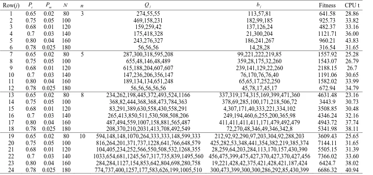
products and different values of the GA parameters are used. Each problem instance has been run 10 times and the minimum fitness value along with its corresponding solution is recorded. Furthermore, CPU t denotes the required CPU time of solving the problem instance.
Table (1): The product data
j
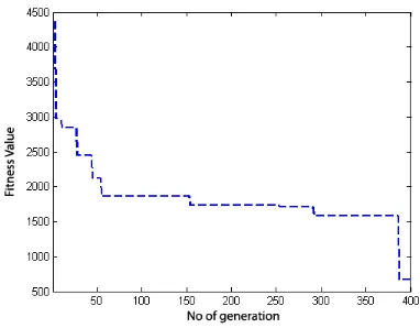
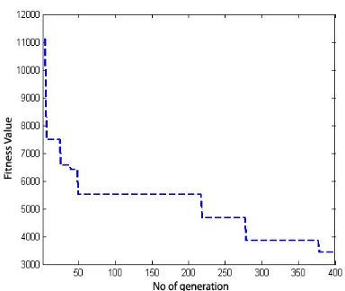
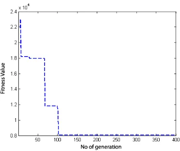
Based on the results of Table (2), when n is selected 3, 5, 8 and 10, the best fitness values are 316.54, 672.94, 3443.9 and 3609.43, respectively. Furthermore, the convergence path graphs of reaching these solutions are presented in Figures (4), (5), (6) and (7), respectively.
17
Figure (6): The convergence path (N=8). Figure (7): The convergence path (N=10).
6.2 Comparison of the fitness evaluation approaches
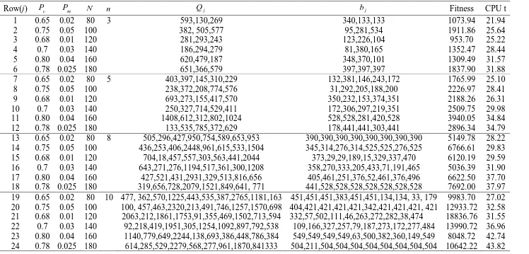
In order to control infeasible solutions, we may employ the penalty policy given by Gen (1997), instead. In this algorithm, the penalty is defined as a positive and known coefficient of violation of constraints (storage capacity and total number of orders). A larger coefficient (penalty) is given to a more infeasible solution; and hence a zero-penalty for a feasible chromosome. In this case, the fitness function of a chromosome is defined as the sum of its objective function and penalty.
The experimental results of employing the penalty policy for the numerical example of section 6.1 are summarized in Table (3). Once more, each row of Table (3), which corresponds to a different problem instance, is run 10 times and the minimum fitness value along with the reorder quantities and the maximum backorder quantities are recorded.
The following conclusions can be made based on the results of Table (3):
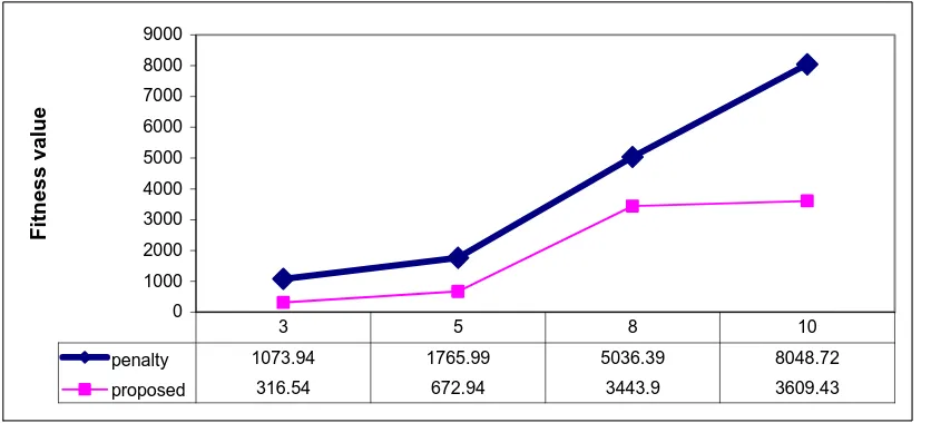
(a) The fitness values of the penalty policy are significantly larger than the ones of the previous approach.
18
Furthermore, based on the results of Table (3), when n is 3, 5, 8 and 10, the best fitness values are 1073.94, 1765.99, 5036.39 and 8048.72, respectively. The convergence path graphs of reaching these results are given in Figures (8), (9), (10) and (11), respectively. Moreover, Figure (12) shows the fitness value graphs of the two fitness evaluation methods.
Figure (8): The convergence path (N=3). Figure (9): The convergence path (N=5).
19
Figure (12): The graph of fitness value for the two fitness evaluation methods (N=3,5,8 & 10).
7. Conclusions and recommendation for future research
In order to make the EOQ model more applicable to real-world production and inventory control problems, in this paper, we expanded this model by assuming several products in which shortages were backordered, the storage had limited capacity and there was an upper bound on the total number of orders. The proposed model of this research applies to a two-level supply chain consisting of a single supplier and a single retailer that operates under vendor management inventory (VMI) system. Under these conditions, we formulated the problem as a non-linear integer-programming (NIP) model and proposed a genetic algorithm to solve it. At the end, a numerical example was presented to demonstrate the application and the performance of the proposed methodology and to compare it to a penalty policy that was applied to fitness evaluation.
For future researches in this area, we recommend the followings:
a) In addition to the storage capacity and the total number of order limitations, we may consider budget and other constraints too.
20
c) Instead of backorder assumption, we can consider lost sale for shortages. Furthermore quantity discounts can be employed.
d) Some of parameter of the model may be either fuzzy or random variable. In this case, the model has either fuzzy or stochastic nature.
e) We can consider multi-echelon supply chains such as; one-retailer multiple-supplier, multiple-retailer single-supplier and multiple-retailer multiple-supplier systems.
8. References
Angulo A, Nachtmann H, Waller MA (2004). Supply chain information sharing in a vendor managed inventory partnership. Journal of Business Logistics, 25: 101–125
Axsäter S (2000). Inventory Control. Kluwer Academic Publishers, Boston, MA, USA
Axsäter S (2001). A framework for decentralized multi-echelon inventory control. IIE Transactions, 33: 91–97
Bertazzi L, Paletta G, Speranza MG (2005). Minimizing the total cost in an integrated vendor-managed inventory system. Journal of Heuristics, 11: 393–419
Biskup D, Simons D, Jahnke H (2003). The effect of capital lockup and customer trade credits on the optimal lot size – a confirmation of the EPQ. Computers and Operation Research, 30: 1509–1524
Cardenas-Barron LE (2001). The economic production quantity (EPQ) with shortage derived algebraically. International Journal of Production Economics, 70: 289-292
Cetinkaya S, Lee CY (2000). Stock replenishment and shipment scheduling for vendor-managed inventory systems. Management Science, 46: 217– 232
21 Table (2): The experimental results of the proposed GA
Row(j) P c P m N n Q j b j Fitness CPU t
1 0.65 0.02 80 3 274,55,55 113,57,81 641.58 28.86
2 0.75 0.05 100 469,158,231 182,99,185 925.73 33.82
3 0.68 0.01 120 159,259,42 137,126,24 482.37 33.16
4 0.7 0.03 140 175,418,328 21,300,204 1121.71 36.00
5 0.80 0.04 160 243,276,327 186,241,267 960.21 43.83
6 0.78 0.025 180 56,56,56 14,28,28 316.54 31.65
7 0.65 0.02 80 5 287,300,318,595,208 99,221,222,219,85 1557.92 25.28
8 0.75 0.05 100 655,48,146,48,489 359,28,175,32,260 1543.07 26.79
9 0.68 0.01 120 615,188,204,607,607 239,141,129,22,260 2188.15 26.7
10 0.7 0.03 140 147,236,206,356,147 76,170,76,76,40 1191.06 30.65
11 0.80 0.04 160 189,134,134,651,248 65,65,17,252,250 1582.02 33.99
12 0.78 0.025 180 56,56,56,56,56 45,78,17,45,17 672.94 34.79
22 Table (3): The experimental results of the penalty policy
Row(j) P c P m N n Q j b j Fitness CPU t
1 0.65 0.02 80 3 593,130,269 340,133,133 1073.94 21.94
2 0.75 0.05 100 382, 505,577 95,281,534 1911.86 25.64
3 0.68 0.01 120 281,293,243 123,226,104 953.70 25.22
4 0.7 0.03 140 186,294,279 81,380,165 1352.47 28.44
5 0.80 0.04 160 620,479,187 348,370,101 1309.49 31.57
6 0.78 0.025 180 651,366,579 397,397,397 1837.90 31.88
7 0.65 0.02 80 5 403,397,145,310,229 132,381,146,243,172 1765.99 25.10
8 0.75 0.05 100 238,372,208,774,576 31,292,205,188,200 2226.97 28.41
9 0.68 0.01 120 693,273,155,417,570 350,232,153,374,351 2188.26 26.31
10 0.7 0.03 140 250,327,714,529,411 172,306,297,219,351 2509.75 29.98
11 0.80 0.04 160 1408,612,312,802,1024 528,528,281,420,528 3940.05 34.84
12 0.78 0.025 180 133,535,785,372,629 178,441,441,303,441 2896.34 34.79
23
Chung KJ, Huang YF (2003). The optimal cycle time for EPQ inventory model under permissible delay in payments. International Journal of Production Economics, 84, 307–318
Cheung L, Lee HL (2002). The inventory benefit of shipment coordination and stock rebalancing in a supply chain. Management Science, 48 (2), 300–306
Chopra S (2003). Designing the distribution networks in a supply chain. Transportation Research, Part E 39, 123–140
Chopra S, Meindl P (2001). Supply Chain Management: Strategy, Planning, Operation, 1st ed., Prentice Hall, Upper Saddle River, NJ, USA
Goldberg D (1989). Genetic Algorithms in Search; Optimization and Machine Learning. Addison-Wesley, Reading, MA, USA
Disney SM, Towill DR (2003). The effect of vendor managed inventory (VMI) dynamics on the bullwhip effect in supply chains. International Journal of Production Economics, 85: 199-215
Disney S M, Towill DR (2002). A procedure for the optimization of the dynamic response of a vendor managed inventory system. Computers & Industrial Engineering, 43: 27–58
Dong Y, Xu K (2002). A supply chain model of vendor managed inventory. Transportation
Research Part E: Logistics and Transportation review, 38: 75-95
Silver EA, Pyke DF, Peterson R (1998). Inventory Management and Production Planning and
Scheduling, 3rd ed., John Wiley and Sons, New York, NY, USA
Mohebbi E (2008). A note on a production control model for a facility with limited storage capacity in a random environment. European Journal of Operational Research, 190, 562–570
Farahani RZ, Elahipanah M (2008).A genetic algorithm to optimize the total cost and service level for just-in-time distribution in a supply chain. International Journal of Production
24
Gen M, Cheng R (2000). Genetic Algorithms and Engineering Optimization. John Wiley and Sons, New York, NY, USA
Goyal SK (1985). Economic order quantity under conditions of permissible delay in payments.
Journal of the Operational Research Society, 36: 35–38
Harris FW (1913). How many parts to make at once? Factory, the Magazine of Management, 10: 135-152
Jaruphongsa W, Cetinkaya S, Lee CY (2004). Warehouse space capacity and delivery time window considerations in dynamic lot-sizing for a simple supply chain. International Journal of
Production Economics, 92: 169–180
Jasemi M (2006). A vendor-managed inventory. Master of Science Thesis, Department of Industrial Engineering, Sharif University of Technology, Tehran, Iran (in Farsi)
Teng J-T (2008). A simple method to compute economic order quantities, European Journal of
Operational Research, 198: 351-353
Kaipia R, Holmstrom J, Tanskanen K (2002). VMI: What are you losing if you let your customer place orders? Production Planning and Control, 13: 17–25
Kleywegt AJ, Nori VS, Savelsbergh MWP (2004). Dynamic programming approximations for a stochastic inventory routing problem. Transportation Science, 38: 42–70
Ko H, Evans G (2007). A genetic algorithm-based heuristic for the dynamic integrated forward/reverse logistics network for 3pls. Computers and Operations Research, 34: 346– 366
Kwak C, Choi JS, Kim CO, Kwon I (2009). Situation reactive approach to vendor managed inventory problem. Expert Systems with Applications, 36: 9039–9045
Lee HL, So, KC, Tang CS (2000). The value of information sharing in a two level supply chain.
25
Lee CC, Chu W, Hung J (2005). Who should control inventory in a supply chain? European
Journal of Operational Research, 164: 158–172
Liao JJ (2007). On an EPQ model for deteriorating items under permissible delay in payments.
Applied Mathematical Modeling, 31: 393–403
Gen M (1997). Genetic Algorithm and Engineering Design, John Wiley & Sons, New York, NY, USA
Magee JF (1958). Production Planning and Inventory Control. McGraw Hill Book Company, New York, NY, USA
Michalewicz Z (1996). Genetic Algorithms + Data Structures = Evolution Programs. 3rd ed., Springer-Verlag, Berlin, Germany
Moinzadeh K (2002). A multi-echelon inventory system with information exchange. Management
Science, 48: 414–426
Moon C, Kim J, Hur S (2002). Integrated process planning and scheduling with minimizing total tardiness in multi-plants supply chain. Computers and Industrial Engineering, 43: 331–349 Nachiappan S, Jawahar N (2007). A genetic algorithm for optimal operating parameters of VMI
system in a two-echelon supply chain. European Journal of Operational Research, 182: 1433–1452
Papachristos S, Skouri K (2003). An inventory model with deteriorating items, quantity discount, pricing and time dependent partial backlogging. International Journal of Production
Economics, 83: 247–256
26
Pasandideh SHR, Niaki STA (2008). A genetic algorithm approach to optimize a multi-products EPQ model with discrete delivery orders and constrained space. Applied Mathematics and
Computation, 195: 506–514
Pentico DW, Drake MJ, Toews C (2009). The deterministic EPQ with partial backordering: A new approach. Omega, 37: 624 – 636
Tersine RJ (1994). Principles of Inventory and Materials Management, 4th ed., Prentice Hall PTR, Englewood Cliffs, NJ, USA
Sofifard R, Hosseini SMM, Farahani RZ (2007). The study of vendor-managed-inventory in supply chain with mathematical model. Master of Science Thesis, Department of Industrial Engineering, Amirkabir University of Technology, Tehran, Iran (in Farsi)
Tyana J, Wee HM (2003). Vendor managed inventory: a survey of the Taiwanese grocery industry.
Journal of Purchasing & Supply Management, 9: 11-18
Van Der Vlist P, Kuik R, Verheijen B (2007). Note on supply chain integration in vendor-managed inventory. Decision Support Systems, 44: 360-365
Vergin RC, Barr K (1999). Building competitiveness in grocery supply through continuous replenishment planning: Insights from the field. Industrial Marketing Management, 28: 145–153
Vigtil A (2007). Information exchange in vendor managed inventory. International Journal of
Physical Distribution & Logistics Management, 37: 131-147
Waller M, Johnson ME, Davis T (1999). Vendor-managed inventory in the retail supply chain.
Journal of Business Logistics, 20: 183-203
27
Woo YY, Hsu SL, Wu SS (2001). An integrated inventory model for a single vendor and multiple buyers with ordering cost reduction. International Journal of Production Economics, 73: 203–215
Xu K, Dong Y, Evers PT (2001). Towards better coordination of the supply chain. Transportation
Research, Part E, 37: 35–54
Yao YL, Evers PT, Dresner ME (2007). Supply chain integration in vendor-managed inventory.
Decision Support Systems, 43: 663–674
Yu YG, Liang L (2004). An integrated vendor-managed-inventory model for end product being deteriorating item. Chinese Journal of Management Science, 12: 32–37 (in Chinese)