Designing Indonesian Liner Shipping Network
Armand Omar Moeis1*, Teuku Yuri Zagoel1, Akhmad Hidayatno1, Komarudin1, Sonny1
Abstract: As the largest archipelago nation in the world, Indonesia’s logistics system has not
shown excellence according to the parameters of logistics performance index and based on logistics costs percentages from overall GDP. This is due to the imbalances of trading on the western and eastern regions in Indonesia, which impacts the transportation systems costs to and from the eastern regions. Therefore, it is imperative to improve the competitiveness of Indonesian maritime logistics through maritime logistics network design. This research will focus on three levels of decision making in logistics network design, which include type of ships in the strategic level, shipping routes in the tactical level, and container allocation in the operational level with implementing butterfly routes in Indonesia’s logistics networking problems. Furthermore, this research will analyze the impact of Pendulum Nusantara and Sea Toll routes against the company profits and percentages of containers shipped. This research will also foresee how demand uncertainties and multi-period planning should affect decision making in designing the Indonesian Liner Shipping Network.
Keywords: Liner network design, maritime logistics, operation research.
Introduction
In 2011, the proportion of Indonesian logistics cost is equivalent to 24.66% of the Gross Domestic Product (GDP). Meanwhile, 11% of the logistics cost are logis-tic transportation costs (Arvis et al. [1], Guericke and Tierney [2], Meeuws et al. [3]). This shows the high cost of logistics in Indonesia. A survey conducted by the World Bank in 2014 stated that Indonesia was ranked 5th on the Logistic Performance Index (LPI) in ASEAN and ranked 53rd from 160 countries around the world. The survey was conducted to assess the performance of each logistics sector in each country by observing the six indicators: process efficiency, infrastructure quality, competitive shipping costs, competence and quality of logistics services, ability to track and trace goods, and travel time (Guericke and Tierney [2], van der Baan [4]).
Indonesia's economic growth in the second quarter of 2015 increased by 4.67%. Spatially, the structure of economic growth in Indonesia is dominated by a group of provinces in Java and Sumatra. Java pro-vides the largest contribution to the Gross Domestic Product (GDP), which is equal to 58.35%, followed by Sumatra that contributes 22.31%, followed by 8.22% from Borneo (Central Bureau of Statistics, 2015). Year to year, Indonesia's economic growth tends to be dominated by Indonesia’s western regions. Th ere-fore, the trend of economic activity, the center of pro-duction, development, and infrastructure develop-ment that mostly occurs in western Indonesia causes a distribution imbalance for the flow of goods between western and eastern Indonesia.
1* Faculty of Engineering, Industrial Engineering Department,
Universitas Indonesia, Kampus Baru Universitas Indonesia, Depok 16424. Indonesia. Email: [email protected]
* Corresponding author
These findings show increased costs of logistics and maritime transportation in Indonesia, resulting in commodity price differrences throughout various regions in Indonesia. With these conditions at hand, opportunities for development and improvement in the field of maritime logistics Indonesia becomes abundant (Agarwal and Ergun [5], Kap and Gunther [6], Cullinane and Khanna [7]).
The imbalance of the flow of goods, increased costs of logistics and transportation is a challenge for stake-holders in the logistics sector, especially the shipping company in the decision process. In designing the network maritime logistics, there are three (3) levels horizon of decision-making: strategic level, tactical level and operational level, where each level will solve the problem of the number and type of vessels, scheduling shipping routes, and the allocation of cargo. We use three types of routes in this research, which are back and forth, butterfly, and pendulum nusantara routes. Bank and forth route is liner shipping routes between 2 ports where ship depart from origin port to destination port and go back again to origin port. Butterfly route is liner shipping route that consist more than 2 ports. Butterfly routes ensure one port will be passed twice (Ronen [8], Meijer [9]). This paper reflects the on going research conducted in our laboratory/research group regard-ing Maritime Logistics topics (Wibowo et al. [10], Moeis and Goputra [11]), particularly Indonesian Liner Network Design (Rahmawan et al. [12], Komarudin et al. [13,14]).
Methods
also inquires profit and operational costs if market demand is to be fulfilled. This research is limited for the main ports of Indonesia, which include Belawan, Tanjung Priok, Tanjung Perak, Makassar, Banjar-masin, and Sorong (van Rijn [15], Smith and Taskin [16]).
Mathematical Model
This research adopts a mathematical model that was developed by Mulder and Dekker [17]. The objective function of this model is maximizing profit and revenue, while minimizing handling costs and trans-shipping costs. This model is then refined by Meijer [9] by adding fuel costs and fixed costs. Furthermore, this research refines the Meijer’s model with adding more variables which are stochastic demand, multi period planning, butterfly routes, and 13 ports. Below is the base model that developed by Mulder and Dekker, refined by Meijer.
Base Model ∈ Indicator set denoting whether port ℎ ∈
is directly visited after port ℎ ∈ on ship route ∈ where = ℎ , ℎ ,
Parameter
ℎ ,ℎ Revenue of transporting one TEU from port ℎ ∈ to port ℎ ∈ .
Cost of transshipping one TEU in trans-shipment port ∈ .
Integer variable that denotes the number of times the route ∈ is used.
ℎ ,ℎ , Direct cargo flow on ship route ∈ between ports ℎ ∈ and ℎ ∈ . ℎ , ,ℎ , Transshipment flow on ship route ∈
between port ℎ ∈ and transshipment port ∈ with destination port ℎ ∈ . ,ℎ, , Transshipment flow on ship route ∈
between Transshipment port ∈ and
Ensure that the total cargo shipped from one port to another does not exceed the demand of that port combination.
∑∈ ∑∈ ℎ , ,ℎ , + ∑ ∈ ℎ ,ℎ , ℎ ,ℎ ℎ ∈ , ℎ ∈
Make sure that the total load of a ship between each two consecutive ports does not exceed the capacity of the ship.
ℎ ,ℎ ,
Ensure that the flow to a Transshipment port with destination port ℎ ∈ has to equal the flow from that Transshipment port to port ℎ .
∑
ℎ ∈� ℎ , ,ℎ ,+ ∑
∈∑
∈ , ,ℎ , ,− ∑
∈ ,ℎ , ,− ∑
∈∑
∈ , ,ℎ , ,= 0
, ℎ , ∈
Define the amount of flow between two consecutive ports.
ℎ ,ℎ ,
− ∑
ℎ ∈�∑
ℎ ∈� ℎ ,ℎ , ℎ ,ℎ ,ℎ ,ℎ ,� ℎ= 0
ℎ , ℎ , ∈
Define the total flow between each two ports in the same cycle.
This model is our refinement/development from base model with adding set of periods. This model can incorporate demand forecasting as necessary input to make better decision in designing Indonesia liner shipping network. ∈ Indicator set denoting whether port ℎ ∈
is directly visited after port ℎ ∈
, Cost of transshipping one TEU in trans-shipment port ∈ for period � ∈ �
Constraints
Below are constrains in this linear programming formulation.
Ensure that the total cargo shipped from one port to another does not exceed the demand of that port combination.
∑∈ ∑∈ ℎ , ,ℎ , , + ∑ ∈ ℎ ,ℎ , , ℎ ,ℎ ,
ℎ ∈ , ℎ ∈ , � ∈ �
Make sure that the total load of a ship between each two consecutive ports does not exceed the capacity of the ship.
ℎ ,ℎ , , ,
ℎ , ℎ , ∈ , � ∈ �
Ensure that the flow to a Transshipment port with destination port ℎ ∈ has to equal the flow from that Transshipment port to port ℎ .
∑ℎ ∈� ℎ , ,ℎ , , + ∑ ∈ ∑ ∈ , ,ℎ , , , − ∑ ∈ ,ℎ , , , − ∑ ∈ ∑ ∈ , ,ℎ , , , = 0
, ℎ , ∈ , � ∈ �
Define the amount of flow between two consecutive ports.
ℎ ,ℎ , , − ∑ℎ ∈�∑ℎ ∈� ℎ ,ℎ , , ℎ ,ℎ ,ℎ ,ℎ ,� ℎ = 0
ℎ , ℎ , ∈ , � ∈ �
Define the total flow between each two ports in the same cycle. demand uncertainty between 2 ports that commonly happen in the real shipping operations where demand cannot precisely be determined (Gram-menos [18]).
∈ Indicator set denoting whether port ℎ ∈ is directly visited after port ℎ ∈ on
Integer variable that denotes the number of times the route ∈ is used.
ℎ ,ℎ , , Direct cargo flow on ship route ∈ between ports ℎ ∈ and ℎ ∈ for scenario ∈ �.
Constraints
Below are constrains in this linear programming formulation.
Ensure that the total cargo shipped from one port to another does not exceed the demand of that port combination.
∑∈ ∑∈ ℎ , ,ℎ , , + ∑∈ ℎ ,ℎ , , ℎ ,ℎ ,
ℎ ∈ , ℎ ∈ , ∈ �
Make sure that the total load of a ship between each two consecutive ports does not exceed the capacity of the ship.
ℎ ,ℎ , ,
ℎ , ℎ , ∈ , ∈ �
Ensure that the flow to a Transshipment port with destination port ℎ ∈ has to equal the flow from that Transshipment port to port ℎ .
∑ℎ ∈� ℎ , ,ℎ , , + ∑ ∈ ∑ ∈ , ,ℎ , , , − ∑ ∈ ,ℎ , , , − ∑ ∈ ∑ ∈ , ,ℎ , , , = 0
, ℎ , ∈ , ∈ �
Define the amount of flow between two consecutive ports.
ℎ ,ℎ , , − ∑ℎ ∈�∑ℎ ∈� ℎ ,ℎ , , ℎ ,ℎ ,ℎ ,ℎ ,� ℎ = 0
ℎ , ℎ , ∈ , ∈ �
Define the total flow between each two ports in the same cycle.
ℎ ,ℎ , , − ℎ ,ℎ , ,
− ∑ℎ ∈� ℎ ,ℎ ,ℎ , , − ∑ ∈ ℎ ,ℎ , , , − ∑ℎ ∈�∑ ∈ ℎ ,ℎ ,ℎ , , , = 0
ℎ ∈ , ℎ ∈ , ∈ , ∈ �
Guarantee a nonnegative flow between each two ports.
ℎ ,ℎ , , 0 ℎ , ℎ , ∈ , ∈ � ℎ ,ℎ , , 0 ℎ ∈ , ℎ ∈ , ∈ , ∈ � ℎ , ,ℎ , , 0 ℎ ∈ , ∈ , , , ∈ , ∈ �
,ℎ, , , 0 ∈ , , ℎ, ∈ , ∈ � , ,ℎ , , , 0 ℎ ∈ , ℎ , , ∈ , ∈ �
Results and Discussions
Model Validation
We validate this model by comparing it with Meijer’s model using the same input. The output comparison between Meijer model and this research model is summarized in Tabel 1.
Back and Forth + Butterfly Shipping Routes Optimization
There are four shipping route combinations in this part. The first route combines butterfly routes with back and forth routes and the second routes incor-porates the first routes with Pendulum Nusantara.
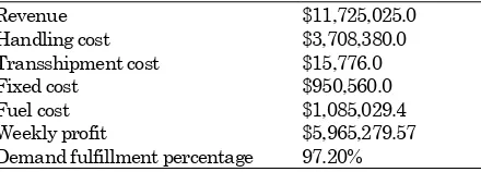
The optimization result of route combination between butterfly routes and back and forth routes using base model as mathematical model can be seen in Table 2 and Figure 1. Figure 1, shows back and forth routes, is the majority in Indonesia liner shipping routes. Demand from and to Sorong must be come from Makassar. It will cause delay for transporting containers from and to Sorong due to many transhipments.
Back and Forth, Butterfly Shipping Routes + Pendulum Nusantara Route Optimization
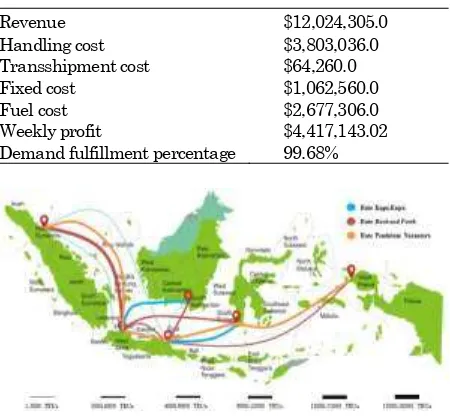
This research also foresees how the Pendulum Nusantara route will affect weekly profits and demand fulfillment percentages. Hence, the route combination in Figure 2 combines the route combi-nations in Figure 1 with the Pendulum Nusantara route. The result is showed in Table 2 and Table 3. In optimal condition, Pendulum nusantara will reduce the weekly profit because Pendulum Nusan-tara is a long route that contributes siginificant number of costs. However, it will increase the percentage of container shipped (97.20% to 99.68%).
Table 1. Output comparison between Meijer model and research model
Metrics Meijer’s Result Research result % Difference Revenue $12,062,300.00 $12,062,350.00 0.00% Handling cost $3,815,072.00 $3,815,072.00 0.00% Fuel Cost $842,165.15 $860,461.58 2.13% Fixed Cost $1,141,000.00 $1,083,560.00 5.30% Profit $6,184,308.85 $6,112,458.42 1.18%
Table 2. Weekly profit calculation for back and forth + butterfly route
Revenue $11,725,025.0
Handling cost $3,708,380.0
Transshipment cost $15,776.0
Fixed cost $950,560.0
Fuel cost $1,085,029.4
Weekly profit $5,965,279.57
Demand fulfillment percentage 97.20% Objective Function
� ∑ℎ ∈ �∑ℎ ∈ �∑ ∈ ∑ ∈ � ℎ,ℎ , ℎ ,ℎ , , + ∑ ∈ ℎ , ,ℎ, , −
∑ℎ ∈ � ℎℎ (∑ ∈ ∑ℎ ∈ �∑ ∈ ∑ ∈ �[ ℎ , ,ℎ , , + ℎ , ,ℎ , , ]+ ∑ℎ ∈ �∑ ∈ �[ ℎ ,ℎ , , + ℎ ,ℎ , , ]) − ∑ ∈ (∑ ∈ ∑ℎ ∈ �∑ ∈ ∑ ∈ ∑ ∈ � , ,ℎ , , , +∑ℎ ∈ �∑ ∈ ∑ ∈ ∑ ∈ � ,ℎ , , , ) −
∑ � − ∑ ∑ ℎ ,ℎ ,�
�,���
Figure 1. Back and forth+butterfly routes illustration
Table 3. Weekly profit calculation for back and forth, butterfly + pendulum route
Revenue $12,024,305.0
Handling cost $3,803,036.0
Transshipment cost $64,260.0
Fixed cost $1,062,560.0
Fuel cost $2,677,306.0
Weekly profit $4,417,143.02
Demand fulfillment percentage 99.68%
Figure 2. Back and forth, butterfly + pendulum routes illustration
Figure 1. Profit comparison between scenario 1 and scenario 2
Optimization using 13 Large Ports in Indo-nesia
This section using 2 scenarios in optimizing Indo-nesia liner shipping problem with 13 main ports. The ports that used are Belawan, Tanjung Priok, Tanjung Perak, Banjarmasin, Makassar, Sorong, Panjang, Palembang, Tanjung Emas, Pontianak, Samarinda, Ambon, dan Bitung. The first scenario is when the liner shipping provider not obligated to fulfill all of demand and the second scenario is when
the liner shipping provider must fulfill all the demand.
Based on the optimization model results of both scenario 1 and scenario 2, the obtained results des-cribe the financial conditions and operations of the company as a substantive consideration in decision making for Indonesian maritime logistics network design. Figure 4 shows the illustration of liner shipping 13 ports without obligation to fulfill all the demand. As the result, there are 5 ports (Palembang, Palembang, Pontianak, Ambon and Bitung) that not served. Figure 5 obligates all the demand to be fulfilled, it will increase the percentage of container shipped but will reduce the profit gained. Figure 3 is a financial performance comparison of shipping companies in scenario 1 and scenario 2 (Rahmawan
et al. [12]). From Figure 3, we can conclude that fulfilling all demand will increase the total revenue, however it will increase the cost as well, especially in fuel cost. As the result, the weekly profit will be slightly decreased.
Figure 2. Illustration of 13 ports scenario 1
Figure 3. Illustration of 13 ports scenario 2
The result from this optimization shows fulfill all the demand will give deduction in profit by 3.6% com-pared with scenario 1. Therefore, not many shipping companies wishing to serve the entire container ports in Indonesia.
Optimization using Multi Period Planning
This research aims to obtain maximum profit for liner shipping companies by including multi period planning. Thus, the initial step is analyzing profit generated in each scenario and each condition. The scenarios are: (1) Fixed number of routes and ships, (2) Fixed number of routes, flexible number of ships, (3)Flexible number of routes and ships. The conditions are: (1) Demand will follow the forecast, (2) Demand will follow the forecast until year 5, then fixed until year 10, (3) Fixed demand. Based on the results of the model, we can see that the 3rd scenario generates the highest profit, compared to the 1st and 2nd scenario, for each condition. Comparison of profit results is shown in the Figure 6 (Komarudin et al.
[13]). 3rd scenario will generate highest profit because this scenario allows the company to adjust the routes and number of ship accordingly based on demand at that year compare to 1st and 2nd screnario.
Next step is to conduct an analysis of fleet allocation for each scenario on each condition. Table 5 shows the comparison of fleet size at the beginning of period.
At the beginning of the period, the 1st scenario has the highest amount of fleet size and the 2nd scenario has the least. The 1st scenario has the highest amount of fleet size because the optimal fleet size must be determined at the beginning of period and will have the same amount on each period. Whereas the 2nd scenario has the least amount because the fleet size is adjusted in accordance to demand on each period. Because the 2nd scenario allows the fleet size to be fixed or increased as the time goes by, based on demand and costs. Comparison of fleet size at the end of period is shown in Table 6.
Table 5. Comparison of fleet size in the beginning of period
1st condition 2nd condition 3rd condition 1st scenario 17 ships 17 ships 16 ships 2nd scenario 13 ships 15 ships 16 ships 3rd scenario 16 ships 16 ships 16 ships
Table 6. Comparison of fleet size in the end of period
1st condition 2nd condition 3rd condition 1st scenario 17 ships 17 ships 16 ships 2nd scenario 18 ships 18 ships 16 ships 3rd scenario 23 ships 21 ships 18 ships
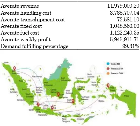
Table 7. Profit calculation with demand uncertainties between ports
Averate revenue 11,979,000.20
Averate handling cost 3,788,707,04 Averate transshipment cost 73,581.10
Averate fixed cost 1,048,560.00
Averate fuel cost 1,122,240.35
Averate weekly profit Demand fulfilling percentage
5,945,911.71 99.31%
Figure 5. Illustration of containers flow with demand uncertainties
Optimization using Demand Uncertainties
The optimization result using back and forth routes with demand uncertainties (Komarudin et al. [14]), can be seen in Table 7 and Figure 7.
It is logical to say that the routes being used in stochastic model is better because it could tackle various conditions of container demand than the predetermined routes model. It gives a strong proof that using stochastic model from the beginning would be more beneficial for liner shipping company. The different routes being used in predetermined routes and stochastic model is shown in Figure 7.
The difference lies on the route between Tanjung Perak and Banjarmasin. Stochastic model shows that it is better to use bigger ship on that route (Panamax 2400) compare to predetermined routes use Panamax 1750. This result further confirmed that it is more beneficial for liner shipping companies to use stochastic model from the beginning as it generates better routes.
Conclusion
volatility and come up with robust solution to integrate that, and (4) serving all of containers demand will give less profit than not serving all of the demand. It can become a national plan to decide logistic subsidy.
Daftar Pustaka
1. Arvis, J., Mustra, M., Panzer, J., Ojala, L., and Naula, L,. Connecting to Compete: Trade Logis-tics in the Global Economy, 2016.
2. Guericke, S. and Tierney, K., Liner Shipping Cargo Allocation with Service Levels and Speed Optimization, Transportation Research Part E: Logistics and Transportation Review, 84, 2015, pp.40-60.
3. Meeuws, R., Sandee, H., and Bahagia, N., State of Logistics Indonesia 2013, Jakarta, 2013. 4. van der Baan, C., Meeuws, R., and Sandee, H.,
State of Logistics Indonesia 2015, Jakarta, 2015. 5. Agarwal, R. and Ergun, O., Ship Scheduling and
Network Design for Cargo Routing in Liner Shipping, Transportation Science, 42(2),2008, pp. 175–196.
6. Kap, H.K. and Gunther, H.O. Eds., Container Terminals and Cargo Systems: Design, Opera-tions Management, and Logistics Control Issues. Berlin: Springer Berlin Heidelberg, 2007. 7. Cullinane, K. and Khanna, M., Economies of
Scale in Large Containerships: Optimal Size and Geographical Implications, Journal of Transport Geography, 8(3), 2000, pp. 181–195.
8. Ronen, D., Ship Scheduling: The Last Decade,
European Journal of Operation Research, 71(3), 1993, pp. 325–333.
9. Meijer, J., Creating a Liner Shipping Network Design, Erasmus University Rotterdam, 2015. 10. Wibowo, R., Hidayatno, A., Komarudin, K., and
Moeis, A., Simulating Port Expansion Plans
using Agent based Modelling, International Journal of Technology, 6(5), 2015, pp. 864-871. 11. Moeis, A. and Goputra, A., Container Stacking
Activity Modeling in Jakarta Container Terminal (JCT) with Three Different Stacking Rules Using Discrete Event Simulation Approach, in The International Conference on Logistics and Maritime Systems, 2015, pp. 30. 12. Rahmawan, A., Komarudin, and Angelina, N.,
Indonesian Maritime Logistics Network Optimi-zation Based Mixed Integer Programming, in
International Conference on Mechanical and Electrical Systems, 2016, pp. 127–131.
13. Komarudin, Purba, M.F.C., and Rahman, I., Multi-Period Maritime Logistics Network Opti-mization Using Mixed Integer Programming,
International Journal of GEOMATE, 13(36), 2017, pp. 94-99.
14. Komarudin, Triastika, A., and Rahman, I., Designing Liner Shipping Network in Indonesia with Demand Uncertainty, International Jour-nal of GEOMATE, 13(36), 2017, pp. 87–93. 15. van Rijn, L., Service Network Design for Liner
Shipping in Indonesia, Erasmus University Rotterdam, 2015.
16. Smith, J. and Taskin, Z., A Tutorial Guide to Mixed Integer Programming Models and Solution Techniques, in Optimization in Medicine and Biology, G.J. Lim and E.K. Lee, Eds. London: Auerbach Publications, 2008, p. 521.
17. Mulder, J. and Dekker, R., Methods for Strategic Liner Shipping Network Design, European Journal of Operation Research, 235(2), 2014, pp. 367–377.