International Review of Economics and Finance 9 (2000) 181–192
Evaluating the Fisher effect in long-term
cross-country averages
Lee Coppock
a, Marc Poitras
b,*
aDepartment of Economics, Hillsdale College, Hillsdale, MI 49242, USA
bDepartment of Economics and Finance, University of Dayton, Dayton, OH 45469-2240, USA
Received 8 February 1999; accepted 23 August 1999
Abstract
This article uses long-term cross-country data to examine the Fisher hypothesis that nominal interest rates respond point-for-point to changes in the expected inflation rate. The analysis employs bounded-influence estimation to limit the effects of hyperinflation countries such as Brazil and Peru. Contrary to the results in Duck (1993), the present evidence does not support a full Fisher effect. By extending the empirical model to account for cross-country differences in sovereign risk, we find evidence consistent with the idea that interest rates fail to fully adjust to inflation due to variation in the implicit liquidity premium on financial assets. 2000 Elsevier Science Inc. All rights reserved.
JEL classification:E40
Keywords:Interest rates; Inflation; Fisher effect
1. Introduction
Irving Fisher postulated that changes in expected inflation leave the real interest rate unaltered by inducing equal changes in the nominal interest rate. The well-known Fisher effect has important implications for the behavior of interest rates and the rationality and efficiency of financial markets. For these reasons, Fisher’s hypothesis has inspired a considerable amount of empirical research. Most of the many studies published during the past several decades have failed to detect a full Fisher effect. Instead, interest rates appear generally to adjust by less than point-for-point in response
* Corresponding author. Tel.: 937-229-2419.
E-mail address: [email protected] (M. Poitras).
to changes in expected inflation. This evidence leads many authors to conclude that financial markets suffer from money illusion.1
Since studies typically focus only on the short-run, their inability to detect a full Fisher effect is perhaps not surprising; as Fisher himself emphasized, the adjustment of nominal rates can be expected to occur only in the long-run (Fisher, 1930). Recently, however, a number of studies have undertaken to test the hypothesis in the long-run, and have found support for a full Fisher effect. In particular, Duck (1993) finds evidence of a full Fisher effect by using long-term averages of inflation and interest rates for a cross section of countries.2
In this article, we reexamine the Fisher effect in long-term cross-country averages. Our analysis employs bounded-influence estimation to limit the effects of influential outliers and obtain results that are robust to small changes in the sample used for estimation. In particular, the bounded-influence techniques serve to limit the effects on the parameter estimates of hyperinflation countries such as Brazil and Peru. In contradiction to the results in Duck (1993), our estimates reject the hypothesis that government bond rates display a point-for-point Fisher effect; we find instead only partial adjustment of interest rates.
Section 2 describes the data and the empirical techniques. Among other things, we argue that testing the Fisher effect by using long-term averages might adhere more closely to economic theory than do commonly used long-run techniques such as cointegration analysis. Section 3 presents the results, and section 4 extends the empiri-cal model to test a hypothesis about the source of partial adjustment. Specifiempiri-cally, we find that the interest rate response depends on the riskiness of the bonds; the tests reject a full Fisher effect only for those countries with sovereign ratings of investment grade. The result concurs with the Fried and Howitt (1983) theory that financial assets feature a liquidity premium that increases with expected inflation.
Finally, in section 5 we offer concluding remarks. In particular, we note that our results imply that increasing the liquidity of government securities can lead to greater stability of interest rates in the face of fluctuating inflationary expections.
2. Data and econometric issues
The data consist of 13-year averages of annual rates of inflation and interest from 1976–1988 for a cross-section of 40 countries.3The empirical model takes the form
ri5 a 1 b0pi1 b1VPi1 et. (1)
For countryi,pirepresents the average annual inflation rate, measured by the gross national product (GNP) or the gross domestic product (GDP) deflator;riis the average short-term or medium-term rate on government debt; and VPi is the variability of inflation, measured by the standard deviation of the annual inflation rate.
bond’s real maturity value is a convex function of the price level. Hence, to maintain the equilibrium real return, the nominal rate must decline. Less formally, Friedman and Schwartz (1982) argue that inflation variability can erode yields by impairing capital market efficiency and thus lowering average real productivity.4
For the purpose of testing the Fisher effect, long-term cross-country averages offer some distinct advantages. First, the Fisher effect cannot be expected to hold in the short-term because typical short-run macroeconomic models determine the inflation rate and the nominal interest rate endogenously. Hence, the observed short-term correlation between inflation and interest rates depends on the paths of the exogenous variables forcing the system. For instance, temporary productivity shocks might induce positive correlation between inflation and interest rates, but liquidity shocks would tend to cause negative correlation.5 Only in the long-run can theory make clear predictions about the response of nominal rates to changes in inflation because the long-term inflation rate can be treated as exogenous with respect to interest rates. Conventional time series studies that test only for short-term correlations have there-fore no direct relevance to Fisher’s hypothesis.6
Additionally, short-run empirical models face the difficulty of measuring expected inflation. Numerous studies employ actual inflation as a proxy for expected inflation, but as Honohan (1985) and Graham (1988) demonstrate, this approach can create substantial errors-in-variables bias. Measurement error does not pose the same prob-lem when the data consist of long-term averages: the Law of Large Numbers implies that short-term errors tend to cancel out when computing long-term averages.7
Several recent studies of the Fisher effect shift focus to the long-run by employing cointegration analysis.8This approach, however, requires the assumption that inflation and nominal rates follow unit root processes. The unit root assumption contradicts economic theory since virtually the entire spectrum of macroeconomic models specifies or predicts a covariance stationary inflation rate.9Nor can empiricism alone settle the issue, since tests for unit roots have essentially zero power against plausible alternatives (Cochrane, 1991). By contrast, the analysis in this article requires no assumption of unit roots. In fact, the method of long-term averages has the advantage of remaining valid in the both the unit root and no unit root cases.10
The foregoing considerations favor the use of long-term averages to test the Fisher effect. A cause for concern, however, is that the empirical model in Eq. (1) might suffer from bias due to omitted variables. Many factors can cause real interest rates to vary across countries.11Here, we mention three possible omitted factors that could cause bias if they correlate with inflation. First, some countries impose controls on interest rates, causing observed rates to deviate from market-clearing rates. Second, tax rates on interest income vary across countries, and a higher tax rate implies a greater marginal effect of inflation on the interest rate. Finally, government bonds of various nations possess differing liquidity and risk characteristics. Liquidity can influ-ence not only real yields, but also the marginal effect of inflation through a Fried-Howitt effect, as discussed below. For this reason, we extend the empirical model in section 4 to account for variation in risk and liquidity.
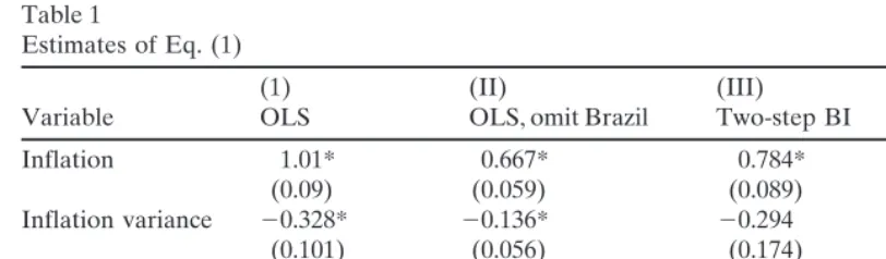
Table 1
Estimates of Eq. (1)
(1) (II) (III) (IV)
Variable OLS OLS, omit Brazil Two-step BI Krasker-Welsch BI
Inflation 1.01* 0.667* 0.784* 0.633*
(0.09) (0.059) (0.089) (0.053)
Inflation variance 20.328* 20.136* 20.294 20.105**
(0.101) (0.056) (0.174) (0.050)
Intercept 2.65** 5.36* 4.88* 5.54*
(1.21) (0.69) (0.81) (0.59)
R2 0.851 0.880 0.713 0.898
owi 40 39 36.72 36.18
Parentheses contain standard errors. The reportedR2applies to the weighted dependent variable.
* Indicates significant difference from zero at the 0.01 level. ** Indicates significant difference from zero at the 0.05 level.
such as Brazil, Bolivia, and Peru; these extreme observations are likely candidates for outliers since empirical regularities that exist under conditions of moderate inflation may break down under conditions of hyperinflation. The magnitude of the hyperinfla-tion observahyperinfla-tions could permit them in a small sample to exert considerable leverage on the parameter estimates. The results in Table 1 show that individual observations can in fact have a pivotal effect on the estimates.
The first two columns of Table 1 present Ordinary Least Squares (OLS) estimates of Eq. (1). The estimates in column I use the full data set, while those in column II omit Brazil, the highest inflation country. The results using the full data set support those of Duck (1993). The point estimate ofb0, the marginal effect of inflation, lies quite close to one, and we cannot reject the hypothesis of a point-for-point Fisher effect. In contrast, column II shows that omitting Brazil reduces the estimate of b0 significantly below one at the .01 level. Hence, the statistical inference on the Fisher hypothesis hinges on whether the sample includes Brazil. Other high inflation countries also exert substantial influence on the estimates.12
To limit the effects of influential outliers, we want to apply a formal technique rather than to arbitrarily discard observations. The bounded-influence (BI) techniques presented by Welsch (1980), and Krasker and Welsch (1982), implement a weighting scheme to yield estimates that do not pivot on a small subset of the data. Welsch (1980) demonstrates a two-step BI technique, while Krasker and Welsch (1982) present an iterative procedure. To explore the robustness of results across techniques, the next section presents both two-step and iterated BI estimates.
3. Bounded-influence methods and results
The BI technique amounts to a kind of weighted least squares with the weightswi satisfying [Eq. (2)].
The BI technique defines the weights according to [Eq. (3)]
wi5 min {1,a/ti}, (3)
wherea is a constant chosen to set the bound on the influence, and tiis a measure of the influence of observationi.13The two-step Welsch and iterative Krasker-Welsch techniques use somewhat different methods to measure the influence, ti. In either case, however, the definition ofticonsists of a quadratic functiond(xi) of the explana-tory variables that measures the “leverage” of observationi, multiplied by a standard-ized measure of the estimated residual for observationi. Thus, we have [Eq. (4)]14
ti5d(xi)|(yi2xibˆ )/s|. (4)
The two-step procedure performs OLS in the first stage and weighted least squares in the second stage. The Krasker-Welsch iterative procedure updates the estimates of b, wi, and s at each step. The procedure converges to a unique solution, and the resulting estimator is consistent and asymptotically normal. The Krasker-Welsch estimator is also asymptotically efficient among BI estimators, given that an efficient BI estimator exists.15 The BI technique does not provide a panacea for all possible econometric pathologies, but the method does yield inferences robust to small sample changes and likely mitigates the effects of omitted variables and data reporting errors. Given the size of our sample, the BI technique insures that any subsample of meaning-ful size should yield essentially the same inferences.
Columns III and IV of Table 1 display BI estimates of Eq. (1). In contrast to the OLS results, the BI estimates ofb0lie significantly below one at the .01 level, indicating rejection of the Fisher hypothesis. The rejection is especially strong in light of the fact that full adjustment with interest taxation impliesb0greater than one. The results contradict those of Duck (1993), and demonstrate the importance of bounding the influence of the outliers in these data. While the results do not support a point-for-point Fisher effect, the estimates do indicate a significant partial effect.16
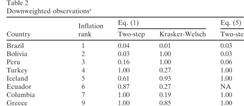
Table 2 lists the downweighted observations and the values of the weights,wi, for the squared residuals. The two techniques can generate different weights because they define the influence differently. Note that the set of downweighted observations almost exclusively includes high-inflation countries; the two-step procedure down-weights five of the six highest-inflation observations, and the iterative procedure downweights six of the nine highest. In particular, both methods strongly downweight Brazil, suggesting that this observation does not conform to the same empirical model as do the bulk of the data.
In the following section we present a brief discussion of some leading theoretical explanations for the failure to observe a full Fisher effect. We then extend the empirical model to examine a theory that attributes the source of partial adjustment to the liquidity properties of financial assets.
4. Sources of partial adjustment
Table 2
Downweighted observationsa
Eq. (1) Eq. (5)
Inflation
Country rank Two-step Krasker-Welsch Two-step Krasker-Welsch
Brazil 1 0.04 0.01 0.03 0.02
Bolivia 2 0.03 1.00 0.03 1.00
Peru 3 0.16 1.00 0.06 0.06
Turkey 4 1.00 0.27 1.00 1.00
Iceland 5 0.61 0.93 1.00 1.00
Ecuador 6 0.87 0.27 NA NA
Columbia 7 1.00 0.19 1.00 0.34
Greece 9 1.00 0.85 1.00 1.00
Spain 14 1.00 1.00 1.00 0.71
Trinidad & Tobago 17 1.00 1.00 1.00 0.73
Guatemala 18 1.00 0.69 NA NA
Denmark 29 1.00 0.97 1.00 1.00
Switzerland 39 1.00 1.00 1.00 0.99
aCountries are ranked from highest (1) to lowest (40) level of inflation. The weights are those assigned
to the squared residuals in least squares estimation.
even in the long-run. A number of authors invoke money illusion, but this explanation conflicts with the fundamental rationality assumption of modern theory. Some hypoth-eses consistent with rationality state that inflation systematically reduces the real interest rate. Most frequently cited is the Mundell-Tobin effect, whereby inflation causes substitution of capital for money, and the resulting increase in the capital stock reduces the real rate. The Mundell-Tobin effect, however, seems unlikely to have an empirically significant effect on interest rates. Summers (1983) calculates that since money holding amounts to less than 2% of the value of the capital stock, substitution of capital for money can reduce the real rate by no more than about 6 basis points. Another explanation for partial adjustment, the so-called Wicksell effect, maintains that redistribution caused by monetary expansion systematically reduces the real rate (Wicksell, 1907; Cagan, 1980). Our calculations indicate that, like the Mundell-Tobin effect, the Wicksell effect cannot account for significant reductions in real rates because of the relatively large size of the existing capital stock.
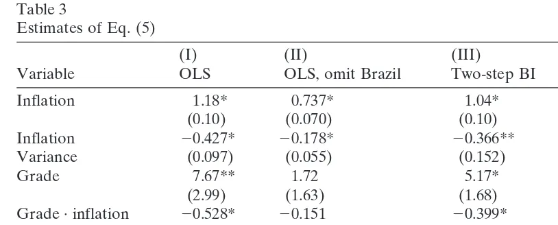
Table 3
Estimates of Eq. (5)
(I) (II) (III) (IV)
Variable OLS OLS, omit Brazil Two-step BI Krasker-Welsch BI
Inflation 1.18* 0.737* 1.04* 0.961*
(0.10) (0.070) (0.10) (0.095)
Inflation 20.427* 20.178* 20.366** 20.316*
Variance (0.097) (0.055) (0.152) (0.068)
Grade 7.67** 1.72 5.17* 4.51*
(2.99) (1.63) (1.68) (1.59)
Grade · inflation 20.528* 20.151 20.399* 20.332*
(0.177) (0.097) (0.106) (0.102)
Intercept 20.85 4.83* 1.58 2.20
(2.44) (1.37) (1.45) (1.38)
R2 0.899 0.925 0.872 0.929
Rwi 35 34 32.12 31.85
Parentheses contain standard errors. The reportedR2applies to the weighted dependent variable.
* Indicates significant difference from zero at the 0.01 level. ** Indicates significant difference from zero at the 0.05 level.
liquidity. In some nations, precious metals or U.S. dollar-denominated assets might supersede sovereign debt as a substitute for money balances in times of inflation.
To control for liquidity differences, we define a dummy variableGRADE taking the value 1 for countries with Moody’s bond risk ratings of investment grade (Baa or higher) and zero otherwise. Strictly speaking, risk and liquidity are not identical; nonetheless, sovereign risk ratings should provide a useful proxy since low risk typically characterizes highly liquid assets.
The extended empirical model takes the form
ri5 a 1 b0pi1 b1VPi1 b2GRADEi1 b3GRADE ·pi1 et. (5)
To allow for a Fried-Howitt effect, the interaction term GRADE · pi permits the marginal effect of inflation on investment grade debt,b01 b3, to differ from that on non-investment grade debt, b0. The specification also includes the dummy variable GRADEto permit a fixed effect, b2, of risk or liquidity on yields.
of the hypothesis of a full Fisher effect for liquid, but not illiquid, sovereigns, which concurs with the Fried-Howitt hypothesis.18
5. Conclusions
For several decades, the empirical literature on the Fisher effect has generally borne an inconsistent relationship to economic theory. While recognizing the theoretical importance of Fisher’s hypothesis, research has often failed to ensure that the implicit assumptions of the empirical model concur with the larger body of economic theory. By analyzing short-term inflation and interest rates, studies have ignored and continue to ignore the endogenous nature of these variables in conventional macroeconomic models. Furthermore, recent studies that do focus on the long-run typically require inflation and nominal rates to follow unit root processes, an assumption inconsistent with the predictions of virtually all macroeconomic models. We find that Duck’s (1993) method of long-term averages frees itself of these shortcomings; however, influential outliers in the data make his results quite fragile. We apply formal techniques to obtain robust estimates and detect only partial adjustment of interest rates.
As international data become more available, the method of long-term averages could be extended to a panel of data consisting of time series of long-term (five- or ten-year) observations on each of several countries. Long-term panel data would permit estimation of a fixed effects model to control for country-specific variation in real interest rates.
Existing literature also fails to derive appropriate theoretical conclusions from empirical rejection of full interest rate adjustment. A plausible interpretation relies on the insight of Fried and Howitt (1983): financial assets yield non-pecuniary liquidity returns that increase with expected inflation. We provide some evidence that concurs with the Fried-Howitt hypothesis.
The Fried-Howitt effect has implications for the monetary integration of Europe. By imposing fiscal discipline and eliminating exchange rate risk, monetary integration should increase the size of the market for debt issues of individual nations. As these assets become more money-like, we can expect liquidity premia to increase and display greater elasticity with respect to shifts in expected inflation. The result implies not only lower interest rates, but also interest rates that are relatively more stable and less sensitive to fluctuations in inflationary expectations. Monetary policy rules that rely on market interest rates to provide information on inflationary expectations would need to adjust to this new environment. Future tests, perhaps using time series methods, could provide more insight on the Fried-Howitt effect in particular, and the functioning of financial markets in general, by testing for a relationship between an asset’s liquidity and the sensitivity of its yield to inflation.
Acknowledgments
Appendix The data
Country Inflation Interest rate Inflation variance Grade
Japan 2.41 6.08 1.96 1
Switzerlanda 2.81 4.43 1.76 1
Germany 3.21 7.35 1.06 1
Netherlands 3.73 8.36 2.65 1
Luxembourga 4.53 8.49 3.19 1
Austria 4.61 8.47 1.28 1
Belgium 4.78 10.24 1.74 1
United States 5.39 9.64 2.32 1
Thailanda 6.03 10.73 5.29 1
Canadaa 6.92 11.10 2.95 1
Tunisia 7.28 7.15 2.37 0
Denmark 7.40 14.69 2.00 1
Francea 7.70 12.40 3.92 1
Pakistan 7.72 9.26 2.62 0
Finland 7.98 8.99 2.30 1
Morocco 7.99 6.38 2.56 NA
Norwaya 8.09 11.16 2.49 1
Sweden 8.26 11.17 1.91 1
Australia 8.61 11.98 1.99 1
United Kingdom 8.95 11.54 4.63 1
Ireland 9.88 13.64 5.18 1
Korea 10.58 9.77 7.67 1
Guatemala 10.98 8.38 8.13 NA
Trinidada 11.11 9.04 3.00 0
Sri Lanka 11.76 12.56 5.71 NA
Venezuela 11.98 12.10 9.40 0
Spain 12.32 8.14 4.46 1
New Zealand 12.66 12.77 3.33 1
Italy 12.72 14.50 4.66 1
South Africa 12.78 13.49 2.58 0
Jamaica 15.03 15.91 6.75 NA
Greece 16.08 18.17 2.81 0
Portugal 18.38 16.57 3.52 1
Columbia 21.80 26.81 2.83 0
Ecuador 21.89 10.58 10.39 NA
Iceland 33.14 23.93 10.89 1
Turkey 36.08 31.13 15.39 0
Peru 51.63 35.94 15.95 0
Bolivia 66.75 38.88 86.56 0
Brazil 68.13 82.40 30.68 0
aIndicates country not included in data published in Duck (1993).
Notes
1. See Modigliani and Cohn (1979), or Summers (1983).
2. See also Evans and Lewis (1995), Pelaez (1995), or Crowder and Hoffman (1996). 3. Appendix A presents the data. Thirty-three of the observations are as reported in Duck (1993). We extend the data by seven countries to increase the power of the tests. The data source is International Financial Statistics, published by the International Monetary Fund.
4. See also the labor supply model of Snow and Warren (1986).
5. Another one of the many sources of short-term correlation of inflation and real rates arises from the notion of uncovered interest parity. Positive monetary shocks lead to short-term depreciation of the domestic currency relative to its long-term level. In this case, the interest rate will be relatively low because of the anticipation that the currency will appreciate and return to its long-term level. 6. Despite these considerations, researchers continue to inappropriately test the Fisher effect only in the short-term; a recent example is the study by Kandel et al. (1996). For a clear discussion of this issue see Summers (1983).
7. The argument from the Law of Large Numbers runs as follows: letutrepresent the short-term expectational error, so that Ept 5 pt 1 ut. Consistent with rational expectations, let ut be iid with mean zero and variance s2u. Then var (n21otpt2n21otEpt)5var(n21otut)5 s2u/n.Hence,n21otpt, the average short-term inflation rate, converges in mean square to n21o
tEpt, the average short-term expectation. Note that statistical forecasts and survey forecasts fail to eliminate the errors-in-variables bias. Fama (1975) averts the errors-in-variables problem by reversing the regression, projecting inflation on the interest rate, but this approach assumes a constant real rate.
8. Examples include Mishkin (1992), Pelaez (1995), and Crowder and Hoffman (1996).
9. An exception is the theory of optimal seigniorage (Mankiw, 1987), but the available evidence strongly contradicts this theory.
10. To demonstrate validity in the unit root case, let inflation follow a simple random walk,pt5 pt211vt, wherevtis white noise. Without loss of generality, let the real interest rate equal zero. Then to compensate lenders for expected inflation, the nominal rate must follow the process rt5 pt21. Thuspt2rt5vt. Computing sample averages yields otpt/n2otrt/n 5otvt/n, which→0 as n→ ∞sincevtis white noise. Hence, for sufficiently largen, the computed averages of inflation and nominal rates move in approximate one-to-one correspondence, as predicted by the Fisher Effect, even with a unit root.
11. If goods are not perfectly mobile, real rates can differ across countries even if financial capital is perfectly mobile. Imperfect mobility of goods implies that investors have little incentive to respond to differentials in real rates of return expressed in terms of the goods of different countries.
the estimated marginal effect back up to 0.76, a shift of more than a full standard deviation.
13. The two-step BI procedure sets a 5 0.34 for approximately 95% asymptotic efficiency. The corresponding figure for the iterated Krasker-Welsch procedure is a 51.596
√
k, withk the number of regressors.14. The Krasker-Welsch technique definess according tocs25n21Siw2i(yi2xibˆ )2, withc5[(n2k)n]Emin(1,a/d2(xi)). Hence,crepresents the average squared weight due to the explanatory variables multiplied by (n 2k)/n. See Krasker and Welsch (1982), and Baum and Furno (1990) for details on the function
d(xi) used in the Krasker-Welsch procedure. The two-step BI estimator defines
ti such that ti 5 |DFFITSi|, where DFFITSi is a standardized measure of the change in the fitted value due to deletion of observation i. By definition, we haveDFFITSi5{hi/(1 2hi)}ui, whereuiis the ith studentized residual, andhi is the ith diagonal element of the ‘hat matrix,’X(X9X)21X9.
15. An efficient BI estimator, however, might not exist.
16. The 33-observation data set used by Duck yields similar results. ReplacingVPi with log(VPi) to allow a diminishing marginal effect of inflation uncertainty on the real rate leaves the results essentially unchanged. Dropping VPi entirely and obtaining BI estimates of the simple regression of nominal rates on inflation also yields similar inferences. In this case, the two-step technique estimates the marginal effect of inflation as .63, while the iterated procedure yields .59. 17. The estimation uses 35 observations because of the unavailability of Moody’s
bond ratings for five countries. For five other countries, bond ratings become available only in 1995, which does not coincide with the relevant period, 1976– 1988. We assume that these observations still reflect ratings during the relevant period since countries infrequently cross the investment grade threshold. 18. The estimates indicate a significantly positive fixed effect ofGRADEon rates,
a result that might reflect correlation of GRADEwith some omitted variable such as marginal capital productivity. Also, Table 2 displays final weights which indicate the influential outliers in the data. The two-step technique strongly downweights the three highest-inflation countries: Brazil, Bolivia, and Peru. The iterative technique strongly downweights Brazil and Peru, and moderately downweights Columbia.
References
Baum, C., & Furno, M. (1990). Analyzing the stability of demand-for-money equations via bounded-influence estimation techniques.Journal of Money, Credit, and Banking 22, 465–477.
Cagan, P. (1980). Comment. In S. Fischer (Ed.),Rational Expectations and Economic Policy(pp. 156–160). Chicago: University of Chicago Press.
Cochrane, J. (1991). Comment. In O. Blanchard & S. Fischer (Eds.),NBER Macroeconomics Annual 1991(pp. 201–210). Cambridge, MA: MIT Press.
Duck, N. (1993). Some international evidence on the quantity theory of money.Journal of Money, Credit, and Banking 25, 1–12.
Evans, M., & Lewis, K. (1995). Do expected shifts in inflation affect estimates of the long-run Fisher relation?Journal of Finance 50, 225–253.
Fama, E. (1975). Short-term interest rates as predictors of inflation. American Economic Review 65, 269–282.
Fisher, I. (1930).The Theory of Interest.New York: Macmillan.
Fried, J., & Howitt, P. (1983). The effects of inflation on real interest rates.American Economic Review 73, 968–979.
Friedman, M., & Schwartz, A. (1982).Monetary Trends in the United States and the United Kingdom.
Chicago: University of Chicago Press.
Graham, F. (1988). The Fisher hypothesis: a critique of recent results and some new evidence.Southern Economic Journal 54, 961–968.
Honohan, P. (1985). Fisher’s paradox: comment.American Economic Review 75, 567–568.
Kandel, S., Ofer, A., & Sarig, O. (1996). Real interest rates and inflation: an ex-ante empirical analysis.
Journal of Finance 51, 205–225.
Krasker, W., & Welsch, R. (1982). Efficient bounded-influence regression estimation. Journal of the American Statistical Association 77, 595–604.
Lucas, R. (1978). Asset prices in an exchange economy.Econometrica 46, 1429–1445.
Mankiw, N. G. (1987). The optimal collection of seigniorage: theory and evidence.Journal of Monetary Economics 20, 337–342.
Mishkin, F. (1992). Is the Fisher effect for real? A reexamination of the relationship between inflation and interest rates.Journal of Monetary Economics 30, 195–215.
Modigliani, F., & Cohn, R. (1979). Inflation, rational valuation, and the market. Financial Analysts Journal 35, 24–44.
Pelaez, R. (1995). The Fisher effect: reprise.Journal of Macroeconomics 17, 333–346.
Snow, A., & Warren, R. (1986). Price level uncertainty, saving, and labor supply.Economic Inquiry 24, 97–106.
Stulz, R. (1986). Interest rates and monetary policy uncertainty.Journal of Monetary Economics 17, 331–347.
Summers, L. (1983). The nonadjustment of nominal interest rates: a study of the Fisher effect. In J.Tobin (Ed.),Symposium in Memory of Arthur Okun(pp. 201–244). Washington, DC: Brookings Institution. Welsch, R. (1980). Regression sensitivity analysis and bounded influence estimation. In J. Kmenta & J.