PROSPECTS OF PHOTON COUNTING LIDAR FOR SAVANNA ECOSYSTEM
STRUCTURAL STUDIES
D. Gwenzi, M.A. Lefsky
Natural Resource Ecology Laboratory, Colorado State University, CO, USA [email protected]
KEY WORDS: Photon counting lidar, ICESat-2, MABEL, Savanna, Canopy height
ABSTRACT:
Discrete return and waveform lidar have demonstrated a capability to measure vegetation height and the associated structural attributes such as aboveground biomass and carbon storage. Since discrete return lidar (DRL) is mainly suitable for small scale studies and the only existing spaceborne lidar sensor (ICESat-GLAS) has been decommissioned, the current question is what the future holds in terms of large scale lidar remote sensing studies. The earliest planned future spaceborne lidar mission is ICESat-2, which will use a photon counting technique. To pre-validate the capability of this mission for studying three dimensional vegetation structure in savannas, we assessed the potential of the measurement approach to estimate canopy height in a typical savanna landscape. We used data from the Multiple Altimeter Beam Experimental Lidar (MABEL), an airborne photon counting lidar sensor developed by NASA Goddard. MABEL fires laser pulses in the green ( 532 nm) and near infrared (1064 nm) bands at a nominal repetition rate of 10 kHz and records the travel time of individual photons that are reflected back to the sensor. The photons’ time of arrival and the instrument’s GPS positions and Inertial Measurement Unit (IMU) orientation are used to calculate the distance the light travelled and hence the elevation of the surface below. A few transects flown over the Tejon ranch conservancy in Kern County, California, USA were used for this work. For each transect we extracted the data from one near infrared channel that had the highest number of photons. We segmented each transect into 50 m, 25 m and 10 m long blocks and aggregated the photons in each block into a histogram based on their elevation values. We then used an expansion window algorithm to identify cut off points where the cumulative density of photons from the highest elevation resembles the canopy top and likewise where such cumulative density from the lowest elevation resembles mean ground elevation. These cut off points were compared to DRL derived canopy and mean ground elevations. The correlation between MABEL and DRL derived metrics ranged from R2 = 0.70, RMSE = 7.9 m to R2 = 0.83, RMSE = 2.9 m. Overall, the results were better when analysis was done at smaller block sizes, mainly due to the large variability of terrain relief associated with increased block size. However, the increase in accuracy was more dramatic when block size was reduced from 50 m to 25 m than it was from 25 m to 10 m. Our work has demonstrated the capability of photon counting lidar to estimate canopy height in savannas at MABEL’s signal and noise levels. However, analysis of the Advanced Topography Laser Altimeter System (ATLAS) sensor on ICESat-2 indicate that signal photons will be substantially lower than those of MABEL while sensor noise will vary as a function of solar illumination, altitude and declination, as well as the topographic and reflectance properties of surfaces. Therefore, there are reasons to believe that the actual data from ICESat-2 will give poorer results due to a lower sampling rate and use of only the green wavelength. Further analysis using simulated ATLAS data are required before more definitive results are possible, and these analyses are ongoing.
1. INTRODUCTION
Lidar remote sensing provides a means to directly estimate the three dimensional biophysical parameters of vegetation using the physical interactions of the emitted pulse with the vegetation structure being illuminated. One widely demonstrated application of lidar has been the estimation of canopy height, which is in turn related to aboveground woody biomass, an important quantity in monitoring carbon storage and dynamics in vegetation systems and central to global carbon cycle studies. Small footprint discrete return lidar (DRL) systems are ideally useful for small extents while large footprint waveform lidar systems are the most ideal for studies at larger extents (Hall et al., 2011). The Geoscience Laser Altimeter System (GLAS) aboard the Ice, Cloud and land Elevation Satellite (ICESat) has been the only available spaceborne lidar sensor and it has provided waveform data with a proven capability to estimate canopy height in various ecosystems (Lefsky, et al., 2007; Duncanson et al., 2010; Xing et al., 2010; Lefsky, 2010; Simard et al., 2011; Gwenzi & Lefsky, 2014a). However, ICESat was decommissioned in 2010 and the earliest planned future mission is its successor, ICESat-2, which will use the Advanced Topography Laser Altimeter System (ATLAS).
Unlike GLAS, that used a full waveform recording technique, ATLAS will use a single photon counting technique. A single photon counting lidar (SPL) system fires thousands of laser pulses per second and records the travel time of individual photons that are reflected back to the sensor. The photons’ time of arrival and the instrument’s Global Positioning System (GPS) position and Inertial Measurement Unit (IMU) orientation are used to calculate the distance the light travelled and hence the elevation of the surface below. The high level of sensitivity of a SPL at low energy expenditure promises extended laser lifetimes and makes it possible to fly at higher altitudes, thus providing a larger coverage. The plan for ATLAS is to use a single pulse which will be split into 6 transmit beams that are arranged in 3 pairs. The configuration will give a distance of 3.3 km between each pair with a 90 m separation between the members of each pair. Using a 10 kHz repetition rate at an altitude of ~500 km will produce footprints of 10 m diameter at 70 cm intervals along track (Abdalati et al., 2010). The primary objective of ICESat-2 will be the quantification of ice sheets and sea ice but just like ICESat-GLAS, vegetation height retrieval for biomass assessment is a science objective, although not a mission requirement.
The Multiple Altimeter Beam Experimental Lidar (MABEL) is an airborne simulator of ATLAS that was developed by NASA Goddard to pre-validate the ICESat-2 mission. MABEL flights were carried out on NASA’s ER-2, a high altitude aircraft (http://www.nasa.gov/centers/armstrong/aircraft/ER-2/index.html). The sensor uses laser pulses in the red (532 nm) and near infrared (1064 nm) wavelengths at a variable repetition rate of 5-25 kHz. Typically, it uses a 10 kHz repetition rate and laser pulse length of 2 ns. At the platform’s nominal speed of 200 ms-1, a pulse will be emitted every 4 cm along the track (McGill et al., 2013). At the ER-2’s operational altitude of 20 km, the laser MABEL configuration are given in (McGill et al., 2013).
The MABEL instrument has been flown aboard the ER-2 on several missions above various earth surfaces between the years 2010 and 2014 at different times of the day. This variation of conditions under which it was flown provides different levels of solar background and other atmospheric conditions necessary to test signal detection algorithms for different surfaces, including vegetation. The aggregation of the time tagged photons along the ground track allows for vertical profiles to be created, on which vegetation and ground elevations can be computed. MABEL was not intended to be an exact duplicate of ATLAS but was meant to provide the measurement concept and data for algorithm development with the flexibility to explore science and engineering trade spaces (McGill et al., 2013). This paper reports work that used MABEL data from one selected channel to generally investigate the prospects of photon counting lidar in retrieving 3-D vegetation structural attributes in a savanna landscape. We hope to provide a base for any other photon counting lidar remote sensing work that aims at calculating canopy height, biomass and consequently carbon storage/dynamics in such ecosystems.
2. METHODS AND MATERIALS
2.1 Study Site
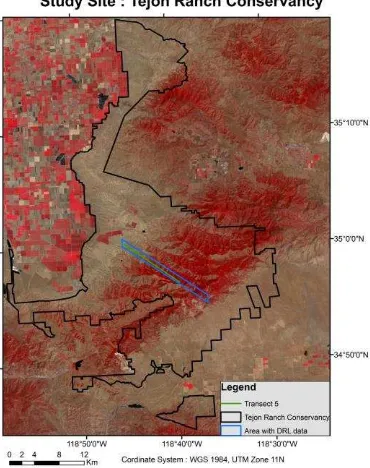
This research was conducted in the oak savannas of Tejon Ranch Conservancy (figure 1). The 2008 Tejon Ranch Conservation and Land Use Agreement between Tejon Ranch Company and a group of conservation organizations resulted in the creation of this 72 000 Ha conservancy. The conservancy was created to protect the ranch and implement science based stewardship, thus preserving, enhancing and restoring the native biodiversity and ecosystem values of the Tejon Ranch and Tehachapi Range for the benefit of California’s future generations (Tejon Ranch Conservancy, 2013). These oak savannas comprise mainly of Blue oaks (Quercus douglasii), Black oaks (Quercus kelloggii) and Valley oaks (Quercus lobata). Other species found in this ecosystem are Canyon live oak (Quercus chrysolepis), Interior live oak (Quercus wislizeni), the California Buckeye (Aesculus californica) and a few conifers. Blue oak woodlands are dominant at the lower elevations (between 500 and 1 000 m), Black oak woodlands are dominant in higher elevation areas (> 1 200 m) while Valley oak woodlands are found on both lower (400- 600 m) and higher (1400- 1800 m) elevations. Grass dominates the understories of Blue and Valley oaks while shrubs are found in
combination with grass in the understory of Black oaks.
2.2 Data
We used data from the February 2012 day time flights. MABEL transects that were coincident with available DRL data were selected for the analysis. For all the transects, we used a single channel (number 49) in the near infrared wavelength since on average it had the highest number of detected photons for the data available. For demonstration and validation purposes, we present the results of one transect (herein referred to as transect 5, shown in figure 1) that had the highest variability in terms of vegetation cover and relief. The height metrics calculated from the MABEL data were validated by comparing them with the equivalent metrics derived from the DRL data. The DRL data was obtained in May 2012 by a commercial lidar vendor at an average density of 1 point per m2 and was validated by field data as explained in (Gwenzi & Lefsky, 2014b).
Figure 1. Map showing Landsat TM false color (432) image of study area and location of DRL data extent and transect 5.
2.3 Height Calculation
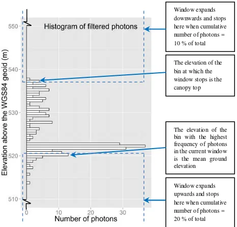
For each transect the channel 49 photons were aggregated at different length segments, herein referred to as blocks. We tested the derivation of canopy height at 3 block lengths (50 m, 25 m, and 10 m). We chose the 10 m block to represent the ICESat-2’s footprint size. The location of the ICESat-2 footprint will be known but the location of any recorded photon within the footprint will be unknown (Rosette et al., 2011). The 25 m block size was chosen to compare with footprint sizes of a prior successful medium resolution lidar sensor, the Laser Vegetation Imaging Sensor (LVIS) and a planned future mission, the Global Ecosystem Dynamics Investigation (GEDI) lidar. We also evaluated the 50 m block size to compare with ICESat-GLAS and determine the effect of analysis at a much coarser resolution. For each block length, the aggregated photons were modeled into a histogram at 0.5 m vertical resolutions according to their elevation above the World Geodetic System (WGS 1984). The raw data for each channel has a lot of noise photons as shown in figure 2. To filter out The International Archives of the Photogrammetry, Remote Sensing and Spatial Information Sciences, Volume XL-1, 2014
much of the noise photons we used only those photons whose elevation was within the µ±2.5σ range for each block. The histogram for each block was used to derive two main height metrics for that corresponding block: Hmax defined as the maximum canopy height minus mean ground elevation and H90 defined as the 90th percentile canopy height minus mean ground elevation.
Figure 2. Transect 5’s raw data
For each block length, we randomly selected a few blocks for which the distribution of the photons showed clear breaks, (i.e. a likely canopy top and ground elevation). These breaks were then matched to the canopy top and mean ground elevation calculated from the DRL data. We related the values for the canopy top and mean ground elevation to the bins of their respective histograms, relative to the highest elevation for canopy top and relative to the lowest elevation for mean ground elevation. From the histograms, we found out that on average for a 50 m block, the break for canopy top corresponded to the elevation of the lowest of the top 10 % photons while that for mean ground elevation corresponded to the elevation of the highest of the bottom 25 % of photons. The corresponding bins for the other block sizes were 10 % and 20 % (25 m) and 5 % and 7.5 % (10 m) for the canopy top and mean ground elevation respectively. Using these results we then implemented an expansion window algorithm (figure 3) in R (R Core Team, 2014) that identified the canopy top and mean ground elevation for every other block for all the block sizes in all transects.
To identify the canopy top, the algorithm starts by drawing a 2 m length window that starts at the highest elevation bin for each histogram and counts the number of photons in that window relative to the total number of photons in the whole histogram. The window then expands by 0.5 m downwards and again counts the number of cumulative photons and the process repeats until the number of counted photons are equal to or greater than the cut off point (i.e. 10 %, 10 %, and 7.5 % for the 50 m, 25 m, and 10 m blocks respectively). The elevation of the bin at which the window stops expanding is therefore the canopy top elevation. For mean ground elevation, the algorithm works the same way but the window starts from the other end of the histogram, i.e. the bin of the lowest elevation and stops at the respective cut off points for the concerned block size. Hmax is therefore calculated as canopy top minus mean ground elevation. For H90 the procedure is almost the same but after identifying the canopy top, and the mean ground elevation, the algorithm then orders the photons in between according to their elevation and identifies the photon at the 90th percent index. H90
will then be calculated as the elevation of the photon at the 90th percent index minus mean ground elevation. To check our algorithm’s ability to derive these height metrics well, we created vegetation profiles along each transect by plotting each block’s canopy top and mean ground elevation at its centre’s coordinates and connect them with a continuous line.
Figure 3. Diagrammatic representation of the height calculation algorithm (an example of a 25 m block from transect 5)
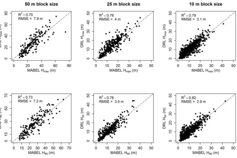
We also checked the accuracy of the height metrics derived from MABEL data by comparing the results of transect 5 to the equivalent metrics calculated from the DRL data along the same transect. To achieve this, we created a 2 m wide polygon through the geographic location of the channel 49 transect to represent the approximate footprint diameter of MABEL. This polygon was then divided into blocks of the same length coincident with those used in MABEL data analysis to extract the validation metrics. From the DRL data we created a Digital Terrain Model and Digital Surface Models (maximum and 90th percentile canopy height) at 2 m resolution using LAStools (Isenburg, 2014). Like with the MABEL data height extraction algorithm, Hmax and H90 for each block were obtained by subtracting the mean ground elevation from the maximum and 90th percentile canopy elevations respectively. We then used the R2 and RMSE statistics to determine the deviation of the MABEL derived metrics from the DRL derived metrics.
3. RESULTS
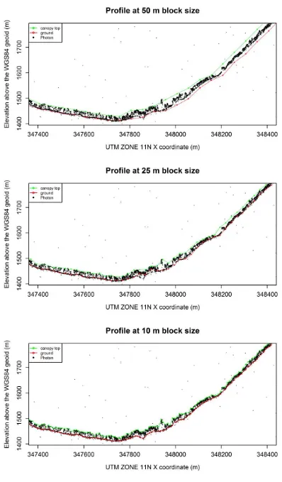
Profiles at the 25 m and 10 m block sizes showed a better representation of the vegetation than those at 50 m, mainly due to limited terrain extents (max-min ground elevation) in the former block sizes compared to the latter. As examples, figure 4 shows the profiles for a 1 km section of transect 5 at the 3 different block sizes and figure 5 shows the validation statistics for the Hmax and H90 metrics for all the blocks within this same transect 5. The H90 height metric was estimated with a slightly better accuracy than the Hmax metric. For both metrics, the results were better when block size was reduced and the increase in accuracy was more dramatic from 50 m to 25 m block sizes than it was from 25 m to 10 m. Grouping the blocks according to the validation residuals and match them with their
Window expands The International Archives of the Photogrammetry, Remote Sensing and Spatial Information Sciences, Volume XL-1, 2014
Figure 4. Examples of profiles at different bock sizes from a 1 km stretch of transect 5
physical locations showed that most of the blocks with the higher prediction errors were on Easterly aspect. From the DRL data and previous field work experience (Gwenzi &Lefsky 2014b), it turned out that Easterly aspect areas generally have sparse vegetation with short height.
4. DISCUSSION
Our algorithm provided encouraging results but were not impressive when compared to other high spatial resolution lidar techniques. We suspect that besides the lower quality of the day time MABEL data, our results could have been affected by the differences in vegetation phenology over the different seasons in which the MABEL and DRL data were collected. MABEL data was collected in February, a season during which the majority of tree species in the study site are leaf off and grass growth is at peak. DRL data was collected in July, a reverse season characterized by leaf on trees and dead grass. The consequences of these differences are twofold: MABEL penetrated more the canopy under leaf off conditions and hence had more ground returns in densely vegetated deciduous tree areas where DRL may not have penetrated well under leaf on conditions. On the other hand, MABEL under leaf off conditions had a higher probability of missing the canopy tips where DRL had higher chances of capturing these tips as surface area is greatly increased by the leaf on conditions. These effects would be compounded because the lower pulse energy of MABEL is less likely to record energy from the very highest elevations and more likely to penetrate to the ground. Moreover
different understory herbaceous vegetation grows over these different seasons in the study area, which can also contribute to the differences in the minimum vegetation heights obtained from each data set.
As with any other georefrenced data, there could be geolocation problems with either the MABEL or DRL data or both. We however do not expect this to have been a big contributor since the profiles drawn by our algorithm were capable of picking well both tree tops and valley bottoms, especially at 10 m block sizes and the DRL data was validated with field data (Gwenzi and Lefsky, 2014b).
Profiles drawn at the 50 m block size do not represent well the vegetation along the transect because of the high heterogeneity of both relief and vegetation within this area. The variability of these two factors is finer than the aggregation length of 50 m. The less dramatic change in accuracy from 25 to 10 m block sizes hints that 25 m is an optimum aggregation length. This concurs with waveform lidar studies where 25 m footprint data from LVIS (Blair et al., 1999; Drake et al., 2002; Anderson et al., 2006) provided better results compared to GLAS data with footprint sizes greater than 50 m in diameter. The generally high prediction error on blocks found on the Eastern aspect is most likely related to the structure of the vegetation. The Easterly aspect in this area is characterized by short and sparse vegetation that is tolerant to the associated drier conditions. Photons that fall on very short and open stands are difficult to discriminate between noise, canopy and ground. This confirms with results from waveform data where we demonstrated that Figure 5. Validation plots for the height metrics at the different block sizes
short height stands on steep terrain pose the main height modeling challenge (Gwenzi & Lefsky, 2014a).
During daylight conditions, part of solar noise may be mixed with valid vegetation returns making it difficult to accurately identify vegetation profiles. Use of night time data with less background noise would have produced better results.
For vegetation studies, we do not expect actual data from ICESat-2’s ATLAS sensor to give better results due to the higher background noise levels and lower sampling rates associated with the larger footprint and use of only the green wavelength. Having few photons in areas that already have low vegetation cover makes it difficult to characterize the vertical distribution of the vegetation at small aggregation blocks. Increasing the aggregation block size will also increase the variability in both relief and tree height. Full waveform lidar has already proven to provide good results for vegetation and the optimum block size of 25 m identified in this work suggests that future missions like GEDI will be a better option than ICESat-2 for canopy height and biomass studies.
Our results are comparable with the few vegetation height reliable biomass estimation since this relationship has been demonstrated well with discrete return and waveform lidar. Rosette at al. (2011) related canopy height simulated from data collected by a photon counting lidar system (Sigma Space’s 3D mapper ) to biomass and reported promising results in a forest area (R2 = 0.72, SE = 53 Mg/Ha).
5. CONCLUSIONS
For such a structurally complex savanna system, the results we obtained are quite encouraging. We however believe that the actual data from ICESat-2 will give poorer results in light of higher background noise, a lower sampling rate and use of only the green wavelength. Given the history of full waveform lidar work, it is our conclusion and recommendation that for vegetation studies, future missions should consider the continued use of full waveform lidar systems such as GEDI. 2 can however be a useful bridge between ICESat-GLAS and any such future waveform lidar mission to ensure continuity of monitoring canopy height, biomass and carbon stocks using spaceborne lidar. waveform lidar to measure northern temperate mixed conifer and deciduous forest structure in New Hampshire. Remote Sensing of Environment, 105(3), pp. 248–261.
Awadallah, M. S., Abbott, A. L., Thomas, V. A., Wynne, R. H., & Nelson, R. F., 2013. Estimating Forest Canopy Height using Photon-counting Laser Altimetry. Silvilaser 2013. Beijing, China.
Blair, J. B., Rabine, D. L., & Hofton, M. A., 1999. The Laser Vegetation Imaging Sensor: a medium-altitude, digitisation-only, airborne laser altimeter for mapping vegetation and topography. ISPRS Journal of Photogrammetry and Remote Sensing, 54(2-3), pp. 115–122.
Drake, J. B., Dubayah, R. O., Knox, R. G., Clark, D. B., & Blair, J. B., 2002. Sensitivity of large-footprint lidar to canopy structure and biomass in a neotropical rainforest. Remote Sensing of Environment, 81(2-3), pp. 378–392.
Duncanson, L. I., Niemann, K. O., & Wulder, M. A., 2010. Estimating forest canopy height and terrain relief from GLAS waveform metrics. Remote Sensing of Environment, 114(1), pp. 138–154.
Gwenzi, D., & Lefsky, M. A., 2014a. Modeling canopy height in a savanna ecosystem using spaceborne lidar waveforms. Remote Sensing of Environment. doi:10.1016/j.rse.2013.11.024.
Gwenzi, D., & Lefsky, M. A., 2014b. Plot level aboveground woody biomass modeling using canopy height and auxiliary remote sensing data in a heterogeneous savanna. Remote Sensing of Environment, (In press).
Hall, F. G., Bergen, K., Blair, J. B., Dubayah, R., Houghton, R., Hurtt, G., … Wickland, D., 2011. Characterizing 3D vegetation structure from space: Mission requirements. Remote Sensing of Environment, 115(11), pp. 2753–2775.
Isenburg, M., 2014. LAStools: award-winning software for rapid Lidar processing.
http://www.cs.unc.edu/~isenburg/lastools/ (01 October 2014).
Lefsky, M. A., 2010. A global forest canopy height map from the Moderate Resolution Imaging Spectroradiometer and the Geoscience Laser Altimeter System. Geophysical Research Letters, 37(15), pp. 1–5.
Lefsky, M. A., Keller, M., Pang, Y., Camargo, P. B. de, & Hunter, M. O., 2007. Revised method for forest canopy height estimation from Geoscience Laser Altimeter System waveforms. Journal of Applied Remote Sensing, 1, 013537.
McGill, M., Markus, T., Scott, V. S., & Neumann, T., 2013. The Multiple Altimeter Beam Experimental Lidar (MABEL): An Airborne Simulator for the ICESat-2 Mission. Journal of Atmospheric and Oceanic Technology, 30(2), pp. 345–352.
R Core Team (2014). R: A language and environment for statistical computing. R Foundation for Statistical Computing, Vienna, Austria. http://www.R-project.org/ (01 October 2014).
Rosette, J., Field, C., Nelson, R., DeCola, P., & Cook, B., 2011. Single-Photon Lidar for Vegetation Analysis. American Geophysical Union Fall Meeting 2011, San Francisco, USA. The International Archives of the Photogrammetry, Remote Sensing and Spatial Information Sciences, Volume XL-1, 2014
Simard, M., Pinto, N., Fisher, J. B., & Baccini, A., 2011. Mapping forest canopy height globally with spaceborne lidar. Journal of Geophysical Research, 116(G04021), pp. 1–12.
Tejon Ranch Conservancy, 2013. Tejon Ranch Conservancy.
http://www.tejonconservancy.org/ (01 October 2014).
Xing, Y., de Gier, A., Zhang, J., & Wang, L., 2010. An improved method for estimating forest canopy height using ICESat-GLAS full waveform data over sloping terrain: A case study in Changbai mountains, China. International Journal of Applied Earth Observation and Geoinformation, 12(5), pp. 385–392.