USING LOGIT MODEL TO IDENTIFY THE DRIVERS OF LANDUSE LANDCOVER
CHANGE IN THE LOWER GANGETIC BASIN, INDIA
I. Mondal a, V.K. Srivastava b, P.S. Roy c, G. Talukdar a
a Wildlife Institute of India, Dehradun, India - (indro.gis, gautamtalukdar)@gmail.com b National Remote Sensing Centre, Hyderabad, India - [email protected]
c Indian Institute of Remote Sensing, Dehradun, India - [email protected]
KEY WORDS: Land Use, Land Cover, Mapping, Change Detection, Interpretation, GIS
ABSTRACT:
The Lower Gangetic Basin is one of the most highly populated areas of India, covering an area of 286,899 km2 with a population density of 720 persons per km2. 64% of the area is covered under agriculture which is supported by the highly fertile alluvial soil. Landuse and landcover (LULC) changes due to an ever increasing human population, natural disasters induced by climate change can alter agricultural productivity which in turn can affect the food security of the region. The current study found out the change in LULC over a span of 20 years (1985-2005), and identified the factors driving this change. LULC data was generated from geo-corrected satellite data of LANDSAT-MSS, IRS LISS-I and IRS LISS-III for pre monsoon and post monsoon seasons for the years 1985-86, 1994-95 and 2004-05 respectively, using onscreen visual interpretation at 1:250,000 scale. We used cross-tabulation matrix to investigate landuse and landcover transformation. The most significant transformation has been to built-up category, contributed by agricultural land (515 km2) and scrubland (53 km2). The other notable transformations are from agriculture to plantation (247 km2), fallow to scrubland (838 km2) and from water body to scrubland (407 km2). We generated change no-change matrix and analyzed it using logistic regression to investigate the drivers of LULC change. We identified availability of water for irrigation, literacy, sex-ratio and the availability of different sources of livelihoods, as the major drivers of LULC change in the Lower Gangetic Basin.
1. INTRODUCTION
1.1 Landuse Landcover studies
Landuse Landcover (LULC) studies have become an important tool to study global environmental change (Liu et al., 2003) and (Giest and Lambin, 2001). LULC change is closely related to biogeochemical cycles and sustainable exploitation of resources (Lambin and Ehrlich, 1997), (Watson et al., 2000) and (Meyer and Turner, 1994)). Scientific research programs, initiated and promoted by the International Geosphere Biosphere Programme (IGBP) and the International Human Dimension Programme (IHDP) in 1995 has further made the study of LULC change a hot topic related to global environmental change (Turner, 1995). Comparisons between the processes, patterns and the dynamics of landuse change at regional scales are key components of LULC study (Turner, 1993).
LULC studies so far conducted in India have primarily catered towards base line data for regional planning and evaluation. There are very few national spatial databases enabling the monitoring of temporal dynamics of agricultural ecosystems, forest conversions, and surface water bodies etc. These kinds of databases are primarily important for national accounting of natural resources and planning at regular intervals. In this context the census of natural resources - land, water, soils, forests and other elements – conducted in a systematic manner and with a repeat cycle to depict changes and modifications as a “snap-shot” of the country’s status of natural resources. The above inventory studies have been carried on under various programmes by the Indian Space Research Organization (ISRO) since 1983 (Ministry of Rural Development, 2010), (FSI, 2011), (Agrawal et al., 2003), (Stibig, 2007), (Roy et al., 2004), (Roy et al., 2000), (Rao, 1996), (Anonymous, 2005) and (Anonymous, 2010).
1.2 Drivers of LULC change
The analysis of Landuse change revolves around the questions; “what drives / causes Landuse change” and “what are the impacts
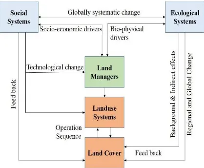
(environmental and socio-economic) of Landuse change”. The “drivers” or “determinants” or “driving forces” of Landuse change are in general belonging either to bio-physical or socio-economic categories (Figure 1).
Figure 1: Relationship between bio-physical, socio-economic drivers and LULC system (after Briassoulis, 1988)
environment. Some of the examples of proximate sources of change are biomass burning, fertilizer applications, species transfer, ploughing, irrigation, drainage, livestock, pasture improvement etc.
1.3 Study area
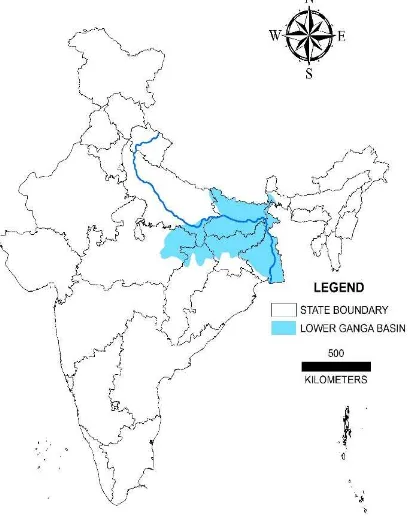
The Lower Gangetic Basin (LGB) is one of the most highly populated areas of India. It extends over an area of 286,899 km2 and cover the states of West Bengal, Bihar and parts of Chhattisgarh, Jharkhand, Madhya Pradesh and Uttar Pradesh. It has a high population density of 720 persons per km2. LGB (Figure 2) is basin number 2A according to the All India Soil & Landuse Survey (AISLUS) Atlas.
Figure 2: Location Map of the Lower Gangetic Basin (LGB)
India being a developing nation, with an ever increasing human population, the impacts of such a populous tract of land on the amount, rate and the intensity of LULC change is very high (Rao, 2001). Such intensified LULC changes has important implications on the sustainable livelihood of the local communities, crop production and environmental change in the region (Semwal et al., 2004).
Any drastic change in the LULC of LGB can alter agricultural productivity of the nation which in turn can affect the food security of the region. So, this study was conducted to investigate the major land transformations that has occurred in this region for the past 20 years and to identify the main drivers of change in the area.
2. MATERIALS AND METHODS 2.1 Datasets
The geo-corrected satellite data of LANDSAT- Multi-Spectral Scanner (MSS), IRS-LISS-I and IRS LISS-III for pre monsoon and post monsoon seasons for the years 1985-86, 1994-95 and 2004-05 respectively was used to study the dynamics of Landuse/ Landcover change. The Landuse / Landcover maps
generated for the period 2004-05 at 1:50,000 scale was degraded to 1: 250, 000. The 1:250,000 scale map of 2004-05 was then used as a base to prepare maps of the previous years.
2.1.1 Data Used
a) IRS LISS – III data of Kharif (August-November), Rabi (December-March) and Zaid (April-June) seasons of 2005-06 b) IRS LISS- I data of 1995(October –December)
c) LANDSAT MSS data of 1985 from January-April and October-November, and
d) LULC maps at 1:50,000 scale prepared under “Natural Resources Census” (NRC) Project of the ‘National Resources Repository’ (NRR) programme of the Department of Space, Government of India.
2.2 Landuse/ Landcover Classification scheme
Landuse and Landcover are not equivalent although they may overlap. Landcover is the physical state of the earth’s surface and immediate subsurface. In other words, Landcover describes the physical state of the land surface: as cropland, mountain or forests. Moser (1996) noted that the term – Landcover originally referred to the type of vegetation that covered land surface, but has broadened subsequently to include human structures, such as buildings or pavement, and other aspects of the physical environment, such as soils, biodiversity, surfaces and ground water. Landuse involves both the manner in which the biophysical attributes of the land are manipulated and the intent underlying that manipulation – the purpose for which the land is used (Turner et al., 1995). Meyer (1996) stated that Landuse is the way in which, and the purpose for which human beings employ the land and its resources. Briefly, Landuse denotes the human employment of land. Skole (1994) expanded further and stated that Landuse itself is the human employment of a Landcover type, the means by which human activity appropriates the results of net primary productivity as determined by a complex of socio-economic factors. Turner (1995) described Landuse as a function or purpose for which the land is used by local human population and can be defined as the human activities which are directly related to land, making use of its resources or having an impact on them. The description of Landuse, at a given spatial level and for a given area, usually involves specifying the mix of Landuse types, the particular pattern of these types, the areal extent and intensity of use associated with each type, the land tenure status. IGBP has accordingly released a classification scheme for Landuse Landcover Change studies. The same classification scheme has been adopted at 1: 250,000 scale (Table 1).
LULC type
(NRC L-I) ( IGBP Classification) Landuse type Code Built up Built up ( both urban and rural) BU
Agriculture Crop landFallow land CLFL
Plantations PL
Forest
Deciduous broad leaf forest DBF
Mixed forest MF
Shrub land SL
Savanna SV
Grassland GL
Permanent wetland PW
Barren / waste
land Barren land Waste land WL BL
Water bodies Water bodies WB
2.3 Generation of Landuse and Landcover Map
The LULC map of 2005 at 1:250,000 scale is primarily derived from 1:50,000 scale NRC-LULC map by hierarchical aggregation of NRC-LULC level 3 and 4 classes to Level 2 classes as per the IGBP-LULC classification scheme. Since our mapping scale was 1:250,000, our minimum mapable unit (MMU) was 562,500 m2. While preparing the NRC-LULC maps, comprehensive ground truth/ checks were already carried out. Further, the aggregation of NRC-LLULC classes to level 2 in the present study has theoretically resulted in a better accuracy as compared to NRC-LULC 1:50,000 scale maps. As the 1995 and 1985 LULC maps are successively prepared by modifying the 2005 and 1995 polygons, respectively, the accuracy of the derived maps of 1995 and 1985 remains close to the ground – verified LULC map of 2005. Nevertheless, areas where major changes have taken place were verified either by visiting the area and conducting local enquiries, or by referring to the government/ official records. The LULC map for the year 2004-05 was treated as the master vector map. A copy of this map was overlaid on the preceding year’s (1994-95) satellite data. The two were registered having uniform projection parameters. The map’s LULC class polygons fell over the same LULC class onto the satellite data. However, the area of the polygons of a LULC class varied. Depending upon the variability, the LULC polygon on the map was edited to generate a new set of polygons. This new edited layer was then considered as the LULC map of 1994-95. Subsequently, the LULC map for 1984-85 was generated using the same methodology.
2.4 Accuracy assessment of LULC data
2.4.1 Classification accuracy: Standard procedure for classification accuracy assessment by (Congalton, 1991) and (Lillesand et al., 2008), which is based on the preparation of error /confusion matrix was used for assessing accuracy. The LULC map of the study area for 2005 has 12 categories for which 50 random points were generated in each category (Congalton, 1988). Ground truthing was done at these locations on the ground. We tried our best to reach these generated location, but where the places were inaccessible, other points falling on the same cover type was taken. Places or LULC types that still could not be captured were done using Google earth. Google Earth imagery with a positional accuracy of 200m (Becek, 2011) served our purpose well as we had a MMU of 740m. Using this, user’s accuracy, producer’s accuracy and overall accuracy was computed.
2.4.2 Change detection accuracy: In order to apply accuracy assessment techniques to change detection, the standard single-date classification error matrix was adapted to a change detection error matrix as proposed by Congalton et al. (1994) and Macleod and Congalton (1998). This new matrix has the same characteristics of the single date classification error matrix, but also assesses errors in changes between two time periods (between time 1 and time 2) and not simply a single classification.
2.5 Change detection of LULC data
A union operation of the vector LULC data of years 1984-85, 1994-95 and 2004-05 was performed in GIS and we used cross-tabulation matrix to investigate landuse and landcover transformation. Major land transformations were then identified and investigated.
2.6 Compilation of driver data
2.6.1 Bio-physical driver data: The bio-physical drivers include characteristics and processes of the natural environment such as weather and climate variables, landform, topography, geomorphic processes, volcanic eruptions, plant succession, soil types and processes, drainage patterns, availability of natural resources. It is important to note that bio-physical drivers do not cause Landuse change directly. They do cause Landcover change which, in turn, may influence Landuse decisions. In addition, Landuse change may result in Landcover changes which, then, feedback on Landuse decisions causing new rounds of Landuse change. The following bio-physical drivers were identified to be used for the current project.
Mean annual rainfall: Rainfall layers at 1/2 degree grid scale for the years 1985, 1995 and 2005, at national level was obtained from IMD. The 1/2 degree grid file was converted into a point file with each point being placed at the centre of each tile, which was then be used in Inverse Distance Weighted (IDW) spatial interpolation technique, for rasterizing the rainfall data. Mean annual temperature: Temperature layer at one degree grid scale for three years 1985, 1995 & 2005 at national level was obtained from Indian Meteorological Department (IMD) as a raster layer.
Distance from roads: Vector road layer was obtained from DCW database and then Euclidean distance was calculated in GIS.
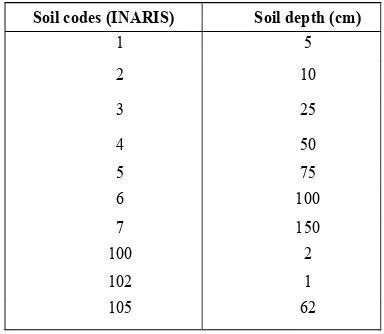
Distance from drainage: The drainage vector layer was obtained from DCW at 1:250,000 scale including rivers and canals. Euclidean distance from drainage was calculated in GIS. Elevation: SRTM data at 90m resolution at national level was used to derive elevation for Lower Ganga Basin. Since the SRTM data is already in raster format it was directly used. Soil depth: The vector soil layer obtained from National Bureau of Soil Survey and Land Use Planning (NBSS&LUP), Nagpur, India, at a scale of 1:250,000, was rasterized using the soil depth values which were assigned according to Table 2.
Soil codes (INARIS) Soil depth (cm)
1 5
Table 2: Soil depth codes according to Integrated National Agriculture Resources Information System (INARIS),
NBSS&LUP
this socio-economic drover data into GIS domain. Then raster layers for each socio-economic driver was generated.
2.7 Logistic regression to analyze the driver of LULC change The interaction among the driver data and LULC change was analyzed using logistic regression analysis. Change was assumed to be a binary variable, where change or no-change per landuse category was considered. For each transformation, we generated 50 random points in areas of change and generated another 50 for areas of no-change. The change in value of the driver variable between two time period t1 and t2 was recorded at these points
using GIS. This binary variable was logistically regressed with different socio-economic and bio-physical drivers, to investigate which drivers were most influential in affecting landuse change. Results of the same, for each investigated transformation, has been explained using the following statistic. “β” indicates the effect size of the explanatory variable on the response variable. The second table describes the model, with χ² indicating how informative the model was compared to the null model. R2N
describes the proportion of information in the response variable explained in the model and the Correct Classification value gives prediction accuracy of the model in terms of predicted versus observed state.
3. RESULTS AND DISCUSSION 3.1 Landuse landcover change
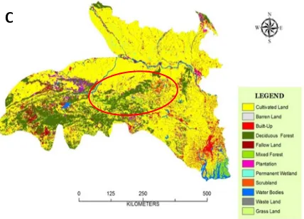
Using the classification scheme, the LULC map of LGB was generated for 1985, 1995 and 2005 using satellite data at 1:250,000 scale (Figure 3). The distribution of various LULC classes and their area statistics was calculated using maps generated for the three time frames (Table 3).
Figure 3: LULC map of 1984-85 (A), 1994-95 (B) and 2004-05 (C). Red circles indicate areas of maximum change.
Crop land is the most dominant LULC class in the lower Ganga basin. The total area under crop land was about 65.42% of the basin’s total geographical area in 1985, which decreased to 64.83% in 1995 and to 64.23% in 2005. On the contrary, fallow land increased from 3.4% in 1985 to 3.68% in 1995 and to 3.88% in 2005. Improving educational and income status may have made people abandon agriculture and move on to other occupations. This shift may have promoted increase in Scrubland at the expense of fallow land. Barren land (BL), Deciduous broad-leafed forest (DBF), grass land (GL) and Mixed forest (MF) show very minute or no change at all.
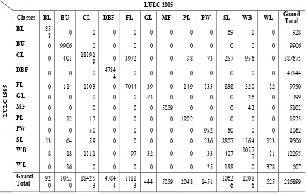
DBF in the study, area mainly occur inside protected. So the change is negligible. Classes like Plantation (PL), Permanent Wetlands (PW) and Scrubland (SL) has shown a very gradual increase in area coverage from 1985 through 2005. Increase in Builtup is very obvious due to increase in size of population and the actual growth in acreage may have been underestimated by the mapping scale adopted. Thereby, it must be noted that although the percentage of built up area is small the increase on its own has been significant. Study area consists of banana, mango, litchi and guava plantation. This is a more profitable form of agriculture. This may account for an increase in area covered by plantation. Water bodies (WB) and waste land (WL) have shown a gradual decrease in area from 1985 to 2005. In the study area, wasteland category is mainly characterized by rocky outcrops. These places are rich in minerals, and are ideal places for setting up mineral mines. We have categorized mining under builtup category. So with increase in mining activity there has been a land transforming from Wasteland to Builtup. In order to understand the dynamics of LULC change during the period of study in the lower Ganga basin, the LULC change dynamic was analyzed (Table 4). The largest amount of transformation is seen from Cultivated Land (CL) to water body (WB) and vice versa (956 and 1111 km2 respectively). This is because of a very
dynamic drainage system in the study area with frequent floods and changes in river course. It is interesting to note that this change from CL to WB and back is balanced. Transition from CL to PL (98 km2) is also large due to agro-forestry practices.
The next significant transformation is from Fallow Land (FL) to Scrub Land (SL), which is about 838 km2. This is obvious
through the natural phenomenon of secondary succession. A similar transformation is from WB to SL (407 km2) and from WL
to SL (118 km2), but this will be due to the process of primary
succession. Another important transformation is the increase in Bulitup (BU), where BU category has acquired acreage from CL (401 km2), FL (114 km2) and SL (53 km2) etc.
A
B
LULC Classes 1985 1995 2005
Area (km2) % of TGA Area (km2) % of TGA Area (km2) % of TGA
Deciduous Forest 47861 16.68 47861 16.68 47861 16.68
Mixed Forest 5096 1.78 5096 1.78 5053 1.76
Scrub 9504 3.31 10075 3.51 10614 3.70
Grassland 400 0.14 434 0.15 447 0.16
Cultivated 187700 65.42 185989 64.83 184264 64.23
Fallow 9743 3.40 10553 3.68 11119 3.88
Plantation 1819 0.63 2001 0.70 2043 0.71
Wetland 1065 0.37 1174 0.41 1455 0.51
Water body 12268 4.28 12036 4.20 12061 4.20
Barren 926 0.32 883 0.31 919 0.32
Wasteland 608 0.21 532 0.19 526 0.18
Builtup 9909 3.45 10264 3.58 10537 3.67
TOTAL 286899 100.00 286899 100.00 286899 100.00
Table 3: Area and percentage area occupied by each LULC category in years 1985, 1995 and 2005. TGA = Total geographical area of the Lower Ganga Basin
LULC 2005
LULC
1985
Classes BL BU CL DBF FL GL MF PL PW SL WB WL Grand Total
BL 85
8 0 0 0 0 0 0 0 0 69 0 0 928
BU 0 9906 0 0 0 0 0 0 0 0 0 0 9906
CL 0
401 181919 0 3972 0 0 98 73 257 956 0 187675
DBF 0 0
0 47844 0 0 0 0 0 0 0 0 47844
FL 0 114 1103 0 7044 39 0 149 133 838 320 12 9750
GL 0 0 0 0 0 373 0 0 0 0 26 0 399
MF 0 0 0 0 0 0 5059 0 0 0 42 0 5102
PL 0 12 12 0 0 0 0 1802 0 0 0 0 1825
PW 0 0 50 0 0 0 0 0 952 60 0 0 1062
SL 53 64 59 0 0 0 0 0 236 8807 164 123 9506
WB 8 18 1111 0 97 32 0 0 33
407 10577 11 12295
WL 0 16 0 0 0 0 0 0 25 188 0 378 607
Grand
Total 920 10530 184253 47844 11113 444 5059 2048 1451 10626 12086 525 286899
Table 4: LULC Change dynamics between year 1985 and 2005. Figures represent area occupied by each LULC class, in km2. BL= Barren Land, BU= Builtup, CL= Cultivated Land, DBF= Deciduous Broadleaf Forest, FL= Fallow Land, GL= Grassland, MF=
3.2 Accuracy assessment
Accuracy assessment of LULC of Lower Ganga Basin for years 2005 was performed whose accuracy has been calculated through the preparation of error matrix. Overall accuracy of Landuse Landcover data for year 2005 was found to be 81%. User’s accuracy and producer’s accuracy was also calculated using this matrix (Table 5). The User’s accuracy of “Waste Land” category was found to be 50%. This is probably the result of confusion between the spectral signatures of wasteland, barren land and scrubland categories.
Category accuracy %User’s accuracy %Producer’s
Barren land 68 91
Table 5: User's and producer's accuracy for LULC categories.
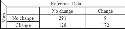
Accuracy assessment for 1995 and 1985 was captured as they were used to calculate the amount of land transformations between 1985 and 2005. Since these images were historical only change detection accuracy assessment was performed. The overall accuracy for year 1995 calculated using this technique was 82.66%. The error matrix is shown in Table 6. Similarly, change detection accuracy assessment was done for year 1985, using the following table, and the overall accuracy was calculated to be 77.16% (Table 7).
Reference Data
Map
No change Change
No change 289 11
Change 93 207
Table 6: Change/no change error matrix of Lower Gangetic Basin for 1995 and 2005
Table 7: Change/no change error matrix of Lower Gangetic Basin for 1985 and 1995.
The trend of decrease in change detection accuracy was logical as the accuracy would keep decreasing with the increase in time difference.
3.3 Logistic regression to analyze the driver of LULC change
After investigating the major land transformation from table 4, we have analyzed the following using logistic regression, to identify the main driver of change.
3.3.1 Fallow to scrubland: The model selected (χ²=119.6, df=3, p<0.001, R2N=0.46) for investigating the drivers influencing this change shows an accuracy of 79%. It indicates rainfall, literacy and elevation as the main drivers. Negative relationship with rainfall (β=-0.442±0.173) indicates that scarce rainfall promotes such land transformation as people are unable to irrigate fallow lands and reuse them for agriculture. It remains fallow until they are colonized by different scrub species. Elevation shows a negative relationship as well (β=-0.854±0.189). In areas with high elevation choice of land for agriculture is limited. So chances are less of people abandoning whatsoever land they have got for agriculture. Literacy has a positive relationship (β=0.764±0.165) i.e., literacy promotes such transformation. It may possible that with increase in literacy people have shifted from a primary occupation like agriculture to tertiary jobs.
3.3.2 Water Body to Scrubland: A 76% accurate logistic regression model (χ²=105.9, df=1, p<0.001, R2N=0.41) shows that rainfall if the main driver for this change and that it has a negative relationship (β=-1.794±0.239). When rainfall decreases, water level in rivers go down exposing sandbars and riverbanks which are fertile alluvial deposits. These areas are quickly colonized by different shrub and grass species.
3.3.3 Fallow to Plantation: The logistic regression model used (χ²=281.9, df=6, p<0.001, R2N=0.85) to investigate this landuse change was 93.7% accurate and it indicated rainfall, literacy and number of establishments as the main drivers. Study area consists of banana, mango, litchi and guava plantation. This is a more profitable form of agriculture. With increase in literacy (β=1.393±0.446) people would want to spend less time in labour intensive agricultural practices and may have invested in plantation crops which are more profitable and require less manual labour the year round. Similar was the effect if people had access to more jobs from commercial establishments (β=2.082±0.583). More rainfall (β=-1.250±0.405) means more available water for irrigation. In that case people may have better chances of growing crops like paddy and wheat which are more irrigation intensive.
4. CONCLUSION
LULC provides a very valuable method for determining the extents of various Landuses and cover types, such as urban, forested, shrubland, agriculture, etc. Such a database enables temporal monitoring of LULC systems like crops, forests, water spread, and waste land reclamation. It can be and has been integrated with climate, socioeconomics, terrain and other variables for the purpose of LULC change modelling. These can further serve as inputs for climate, productivity and biodiversity change models. The LULC database generated here is at a scale of 1:250,000. It serves the purpose of capturing broad changes in Landuse and can be used to locate areas where a finer database needs to be prepared for more detailed investigation and modelling.
ACKNOWLEDGEMENT
REFERENCES
Agrawal, S., et al., 2003. SPOT VEGETATION multi temporal data for classifying vegetation in south central Asia. Current
Science, 84(11), pp. 1440-1448.
Anonymous, 2005. Integrated Resource Information for Desert
Areas. Hyderabad: National Remote Sensing Centre.
Anonymous, 2010. National Land Use and Land Cover Mapping
Using Multitemporal Awifs Data (LULC-AWIFS). Hyderabad:
National Remote Sensing Centre.
Becek, K., Khairunnisa I., and B Barussalam, 2011. On the Positional Accuracy of the Google Earth Imagery. FIG Working
Week 2011, Bridging the Gap between Cultures.
Congalton, R. , R. Macleod, and F. Short, 1994. Developing Accuracy Assessment Procedures for Change Detection
Analysis. Beaufort, NC: NOAA CoastWatch Change Analysis
Program.
Congalton, R.G., 1988. A comparison of sampling schemes used in generating error matrices for assessing the accuracy of maps generated from remotely sensed data. Photogrammetric
Engineering and Remote Sensing, 54, pp. 593-600.
Congalton, Russell G., 1991. A Review of Assessing the Accuracy of Classifications of Remotely Sensed Data. Remote
sensing of Environment, 37(1), pp. 35-46.
Forest Survery of India, 2011. India State of Forest Report.
Dehra Dun: Forest Survery of India, Ministry of Environment and Forest, Government of India.
Geist, Helmut J., and Eric F. Lambin, 2001. What drives tropical
deforestation? LUCC Report series 4, pp. 116.
Lambin, Eric F., and Daniele Ehrlich, 1997. Land-cover changes in sub-Saharan Africa (1982–1991): Application of a change index based on remotely sensed surface temperature and vegetation indices at a continental scale. Remote sensing of
environment, 61(2), pp. 181-200.
Lillesand, T.M., R.W. Kiefer, and J.W. Chipman, 2008. Remote
Sensing and Image Interpretation. John Wiley & Sons, New
York.
Liu, Jiyuan, et al., 2003. Study on spatial pattern of land-use change in China during 1995–2000. Science in China Series D:
Earth Sciences, 46(4), pp. 373-384.
Macleod, R.D., and R.G. Congalton, 1998. A Quantitative Comparison of Change-Detection Algorithms for Monitoring Eelgrass from Remotely Sensed Data. Photogrammetric
Engineering and Remote Sensing, 64(3), pp. 207-16.
Meyer, William B., and B. L. Turner, 1996. Land-use/land-cover change: challenges for geographers. GeoJournal, 39(3), pp.
237-240.
Meyer, William B., and B.L. Turner, (eds), 1994. Changes in
land use and land cover: a global perspective. Vol. 4. Cambridge
University Press.
Ministry of Rural Development, 2010. Wastelands Atlas of
India. Department of Land Resources, Ministry of Rural
Development, Government of India, New Delhi.
Moser, Susanne C., 1996. A partial instructional module on global and regional land use/cover change: assessing the data and searching for general relationships. GeoJournal, 39(3), pp.
241-283.
Rao, K. S., and Rekha Pant, 2001. Land use dynamics and landscape change pattern in a typical micro watershed in the mid elevation zone of central Himalaya, India. Agriculture,
ecosystems & environment, 86(2), pp. 113-124.
Rao, U.R., 1996. Space Technology for Sustainable
Development. Tata McGraw-Hill.
Roy, P. S., and Sanjay Tomar, 2000. Biodiversity characterization at landscape level using geospatial modelling technique. Biological Conservation, 95(1), pp. 95-109.
Roy, P. S., et al., 2004. Biome Level Characterisation of Indian
Vegetation using IRS‐WiFS Data. Indian Institute of Remote
Sensing (National Remote Sensing Agency), Department of Space, Government of India, Dehradun, India.
Semwal, R.L., et al., 2004. Patterns and ecological implications of agricultural land-use changes: a case study from central Himalaya, India. Agriculture, Ecosystems & Environment,
102(1), pp. 81-92.
Skole, David L., 1994. Data on global land-cover change: acquisition, assessment and analysis. Changes in land use and
land cover: a global perspective, pp. 437-471.
Stibig, H. J., et al., 2007. A Land-Cover Map for South and Southeast Asia Derived from Spot-Vegetation Data. Journal of
Biogeography, 34(4), pp. 625-37.
Turner, Billie Lee, et al., 1995. Land-use and land-cover change. Science/Research Plan. Global Change Report, Sweden.
Turner, Billie Lee, Richard H. Moss, and D. L. Skole, 1993. Relating land use and global land-cover change: a proposal for an IGBP-HDP core project. A report from the IGBP/HDP Working Group on Land-Use/Land-Cover Change. Global
Change Report, Sweden.
Watson, Robert T., et al., 2000. Land use, land-use change and forestry: a special report of the Intergovernmental Panel on