BEYOND MAXIMUM INDEPENDENT SET: AN EXTENDED MODEL FOR
POINT-FEATURE LABEL PLACEMENT
Jan-Henrik Haunerta∗ Alexander Wolffb
a
Geoinformatics Group, Institut f¨ur Informatik, Universit¨at Osnabr¨uck, Germany – [email protected] bLehrstuhl f¨ur Informatik I, Universit¨at W¨urzburg, Germany
Commission II, WG II/2
KEY WORDS:Map labeling, point-feature label placement, NP-hard, integer linear programming, cartographic requirements
ABSTRACT:
Map labeling is a classical problem of cartography that has frequently been approached by combinatorial optimization. Given a set of features in the map and for each feature a set of label candidates, a common problem is to select an independent set of labels (that is, a labeling without label–label overlaps) that contains as many labels as possible and at most one label for each feature. To obtain solutions of high cartographic quality, the labels can be weighted and one can maximize the total weight (rather than the number) of the selected labels. We argue, however, that when maximizing the weight of the labeling, interdependences between labels are insufficiently addressed. Furthermore, in a maximum-weight labeling, the labels tend to be densely packed and thus the map background can be occluded too much. We propose extensions of an existing model to overcome these limitations. Since even without our extensions the problem is NP-hard, we cannot hope for an efficient exact algorithm for the problem. Therefore, we present a formalization of our model as an integer linear program (ILP). This allows us to compute optimal solutions in reasonable time, which we demonstrate for randomly generated instances.
1. INTRODUCTION
Maps and technical drawings are usually annotated with textual or pictorial labels in order to help their users understand what they see. A natural requirement to ensure readability is that labels must not overlap. Especially in printed maps where extra infor-mation cannot be added on demand, one usually wants to label as manyfeatures(such as cities, rivers, or countries) as possible. Let’s formalize this problem; thebasic map-labeling problem. Given a set of features and, for each feature, a set of label candi-dates, each with a positive weight, select for each feature at most one label from the set of candidates such that (i) no two selected labels overlap and (ii) the sum of the weights of the selected la-bels is maximized. If a labeling satisfies (i), it is an independent set in the label–label conflict graph that contains a node for each label and an edge for each pair of overlapping labels. For interac-tive applications such as car navigation, this problem is of great importance. For high-quality cartographic purposes, however, we will argue that the above basic problem lacks expressiveness.
First attempts to formalize the rules that govern the labeling of a map have been made in the early 1960s, by Imhof (1975) and Alinhac (1962). First, cartographers (such as Yoeli, 1972), but later also computer scientists tried to automate the tedious pro-cess of labeling maps using heuristics, rule-based or expert sys-tems (Doerschler and Freeman, 1989). Theoreticians focused on apparently simple special cases such as the point-feature label placement problem with four axis-aligned rectangular label can-didates per point, the so-calledfour-position model. According to this model, each label must be placed such that one of its four cor-ners coincides with the point to be labeled. Formann and Wagner (1991) showed that the problem is NP-hard and gave approxima-tion algorithms, which guarantee that a soluapproxima-tion “weighs” at least a certain fraction of an (unknown) optimum solution. Around the same time, researchers such as Zoraster (1986, 1990) started using integer linear programming for map labeling. Many
com-∗Corresponding author
binatorial optimization problems can be expressed as integer lin-ear programs (ILPs). Some of these problems are NP-hard, and hence, so is general integer linear programming. Still, highly op-timized solvers for ILPs are available, and allow the user to solve small- and medium-size instances of many problems quite fast.
Zoraster’s early ILP formulations were later refined by Verweij and Aardal (1999). In order to speed up the computation of optimal or near-optimal solutions, they suggested to employ so-calledcutting plane techniques. Ribeiro and Lorena (2008) pre-sented two ILP formulations and reported that, for instances of 1000 points, “no optimal solution was found in several hours un-til CPLEX [7.5] reached an out-of-memory state”. Therefore, they suggested to use a so-called Lagrangian relaxation based on a clustering of the label–label conflict graph. Combining this La-grangian clustering with the better of their two ILP formulations helped them compute, within about one hour, solutions that were no more than 1.3 % from optimal.
Rylov and Reimer (2014) formulate the basic map labeling prob-lem as an ILP. Additionally, they express the cartographic quality of a labeling and adjust the label weights accordingly. They solve real-world instances using three different general-purpose opti-mization heuristics; namely greedy, gradient descent, and simu-lated annealing. The latter is the slowest method but yields also the best results in terms of quality.
of our extended ILP of more than 1000 labels to optimality, even if the label–label conflict graph is very dense.
2. METHODOLOGY
We start by recalling (see Sect. 2.1) and discussing (see Sect. 2.2) the ILP of Rylov and Reimer (2014), which is the basis of our extensions (see Sects. 2.3–2.5. We discuss how to set up and solve our ILP (see Sect. 2.6).
2.1 A Basic Integer Linear Program
In the basic map-labeling problem, we are given a setF of fea-tures and, for each featuref∈ F, a setL(f)of label candidates. The set of all label candidates isL = S
f∈FL(f). Rylov and Reimer (2014) introduce a 0–1 variable for each label candidate:
xℓ∈ {0,1} for eachℓ∈L . (1)
Since we will later add another group of variables, we refer to the above variables asx-variables. Generally, if a variablexℓ is set to 1, the label candidateℓisselected; it becomes alabel. (For simplicity, in the sequel, by “labels” we will also mean label candidates.) Using these variables, Rylov and Reimer define the following objective function, which aims at selecting a subset of the label candidates of maximum total weight.
MaximizeX ℓ∈L
w(ℓ)·xℓ (2)
They forbid that two overlapping labels are selected by requiring
xa+xb≤1 for eacha, b∈Lwitha6=bandaoverlapsb. (3) If the given labeling instance is such that any two label candidates of the same feature overlap, then Constraint (3) automatically en-sures that any feature receives at most one label. If, however, a feature has label candidates that do not overlap each other, the following constraint needs to be added:
X
ℓ∈L(f)
xℓ≤1 for eachf∈ F (4)
Rylov and Reimer term their ILP formulation a “comprehensive multi-criteria model”. Indeed, the model is quite general since many criteria of cartographic quality can be modeled by specify-ing the weight functionw. We argue, however, that not all criteria of cartographic quality can be expressed with this. Nevertheless, the ILP presented in this section forms the basis for our extended model, which is why we term it thebasic ILP. It hasO(|L|) in-teger variables andO(|L|2)constraints since we may need to
in-stantiate Constraint (3) for each pair of label candidates.
2.2 Disadvantages and advantages of the basic ILP
A shortcoming of the basic ILP is that the weight of a label needs to be defined before solving the ILP and, thus, has to be set with-out knowing which of the other labels are placed. Therefore, the possibility of expressing interdependences between labels is very limited. For example, to judge whether the association between a point labelℓand its corresponding pointpis clear, it is im-portant to know which other points are labeled. This particularly holds if the rule is to display only those points that receive a la-bel: With that rule, only if a pointp′is labeled, a labelℓcan be misinterpreted as the label forp′. We could rule out ambiguous label–point associations by setting up hard constraints similar to Constraint (3), for example, to express that a labelℓmust never be placed together with a label forp′. We argue, however, that
such a constraint would be too strict and that the clarity of asso-ciations should rather be modeled in the objective function. This is not possible with a weighted sum of thex-variables.
A second problem with the basic ILP is that, among two feasible solutionsS1 ⊆LandS2 ⊆LwithS1 ( S2, the solutionS2
containing more labels is always preferred. In other words, if a label can be added to a solution, then this solution cannot be optimal. Consequently, an optimal labeling tends to be densely packed with labels and may occlude the map background almost completely. In fact, in the optimization community, map labeling is referred to as apacking problem(Formann and Wagner, 1991). It is clearly not the objective of map labeling, however, to occlude the map background as much as possible. Therefore, the existing models need to be reconsidered.
Before we turn to an extension of the model, we need to admit that the basic ILP is not as bad as it may seem.
First of all, every subset of an optimal solution to the basic ILP is a feasible solution. Therefore, it can be reasonable to first com-pute an optimal (or a close-to-optimal) solutionS ⊆ Lto the basic ILP, to store this solution, and, at any time, to display only a selectionS′of rectangles fromS, such that the map background is not occluded too much. This two-step approach of first com-puting a densely packed solutionSwithout label–label overlaps and then filteringSto obtain the actual labelingS′is particularly useful for real-time cartography. In this application, labelings need to be computed on the fly and thus the supposedly difficult part of the labeling problem – avoiding label–label overlaps with-out loosing too much information – arguably should be solved in a pre-processing step (Been et al., 2006).
A second argument for the basic ILP is that the occlusion of the map background can be controlled by defining the labels larger than necessary. For example, the label holding a certain text can be defined by buffering the text’s bounding box with a certain distanceε ∈R>0. This in essence means that between any two
displayed texts a minimum distance of2εis ensured. We argue that strictly requiring a minimum distance between two texts is important to ensure the legibility of each label. To avoid that large parts of the map are covered with labels, however, a more global constraint is needed.
2.3 Penalizing ambiguous label–feature associations
In this section we present an extension of the basic ILP to reduce the risk that a user interprets a label of some featurefas the label of a different featuref′. We first discuss this in a general context and then exemplify it for point-feature label placement.
Our model is based on a graphG= (L, E)that contains a node for each label inL. The setE contains an edge between two labelsa, bif placing bothaandbis possible yet undesirable. To express how undesirable it is to place bothaandb, we define a cost functionc:E→R>0. If for an edgee={a, b} ∈Eboth
labelsa, bare selected at the same time, we charge the costc(e), meaning that the objective value is reduced byc(e). For ease of notation, we writec(a, b)forc(e)withe={a, b}. To formalize the idea in linear terms, we introduce continuous variables
ye∈[0,1] for eache∈E , (5)
which we termy-variables. These are linked with thex-variables such thatye= 1if bothxa= 1andxb= 1fore={a, b}:
If at least one of the two labelsa, bis not selected, however, Con-straint (6) does not have any influence on the variableye.
The extended model has the following objective function:
MaximizeX costc(e)is correctly charged ifaand bare selected. Else, if
xa = 0orxb = 0,yeis free within the interval[0,1]; sinceye appears with a negative coefficient in an objective function that we maximize, it will receive the smallest possible value, which is
0, and the costc(e)forewill not be charged. This means that, even though we definedyeas a continuous variable, it will always receive the value0or1in an optimal solution. We conclude that our extended model does not need additional integer variables, which has computational advantages. Since our model has both integer variables and continuous variables it is in fact a mixed integer linear program (MILP).
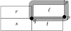
Finally, we suggest a cost functioncwhen labeling points in the four-position model. In this case, we would like to prevent situ-ations such as the one displayed in Fig. 1. In this example, the rectangular labelℓcorresponds to the point p, yet a user may think thatℓis the label forq, sinceqis within a specified distance
ρ∈ R>0fromℓ. Therefore,ℓshould not be displayed together
withq. Assuming thatqis displayed if and only if it receives a label, we can equally well say thatℓshould not be displayed to-gether with one of the labels forq. Since the upper-right label for
qis not possible in conjunction withℓ, we add three edges to the graphG, namely{ℓ, r},{ℓ, s}, and{ℓ, t}. within distanceρfromℓbut alsopis within distanceρfromt.
2.4 Controlling occlusion of the map background
In Sect. 2.2 we argued that the occlusion of the map background could be controlled by defining the labels larger than necessary, for example, by buffering the bounding boxes for the texts that are to be displayed. Because of Constraint (3), this in essence means that any two labels have to be separated with a certain amount of empty space between them. While Constraint (3) acts locally, we may also require that, overall, at most a certain numberKglobal∈ Z>0of labels can be placed. This can be modeled as follows.
X
ℓ∈L
xℓ≤Kglobal (8)
Constraint (8) acts on the entire map and thus on a global level. To control the occlusion of the map background in an adequate way, we introduce a constraint whose region of influence can be ad-justed, such that this more general constraint subsumes both Con-straint (3) and ConCon-straint (8), but also conCon-straints acting somehow between the local and the global level. More precisely, our model relies on the definition of a regionΓ⊆R2. Our idea is to require that every translateγofΓoverlaps at most a certain numberKΓ
of labels. For example, when definingΓas a disk of constant ra-diusδ, our requirement means the following: In the output map, every disk of radiusδoverlaps at mostKΓlabels. By restricting
Γ = {(0,0)}to the origin and settingKΓ = 1, we can avoid overlaps between any two labels and thus achieve the same effect as with Constraint (3). On the other hand, by settingΓ =R2and
ρ
Figure 1: A pointpwith a labelℓ, which can be misinterpreted as the label forq, sinceqis within distanceρfromℓ. When labeling
pwithℓ, the label forqcan ber,s, ort.
Figure 2: A labelℓ, a regionΓ, and the Minkowski difference
M(ℓ) =ℓ⊖Γ. TranslatingΓwith a vector~v ∈M(ℓ)yields a regionγ(~v)overlappingℓ.
KΓ =Kglobal, we allow at mostKgloballabels to be placed in total, which is the same as Constraint (8).
To formalize our requirement in linear terms, a first idea is to define a constraint similar to Constraint (8) for each regionγthat can be obtained by translatingΓ. In other words, we would need one constraint for each possible translation vector~v ∈ R2. Let
γ(~v) = Γ +~v ⊆ R2 be the region obtained by translatingΓ
with~v, and letL(γ)⊆Lbe the set of labels inLoverlapping a regionγ⊆R2. Then, we can express our requirement as follows.
X
ℓ∈L(γ(~v))
xℓ≤KΓ for each~v∈R2 (9)
The problem with this definition is that there are infinitely many vectors in R2, thus it seems that we need an infinite number of instantiations of Constraint (9). This is not the case, how-ever, since for two distinct vectors~v1, ~v2 ∈ R2 it can hold that
L(γ(~v1)) =L(γ(~v2)). In this case, Constraint (9) would clearly be the same for both~v=~v1and~v=~v2, thus we need not instan-tiate it twice. Generally, there can only be2|L|
distinct instantia-tions of Constraint (9), which is a finite (though large) number.
In the following, we assume that the labels as well as the region
Γ ⊆ R2 have constant complexity, for example, they are axis-aligned rectangles (each described with four parameters) or disks (each described with three parameters). We will see that, under these assumptions, the extended model with our general require-ment has the same asymptotic number of constraints as the basic ILP. In the examples that we present in this section, we will use an irregular triangle forΓto show thatΓis not required to be symmetric. Constant complexity of shapes is required, however, to ensure that our ILP has a manageable size.
ℓ1
ℓ2
ℓ3
F1
F2
F3 F5
F4 F
6
F7
Γ x
y
x y
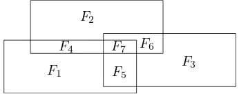
Figure 3: Three labelsℓ1,ℓ2, andℓ3 with their Minkowski dif-ferencesM(ℓ1),M(ℓ2), andM(ℓ3)(top) as well as the facets of the arrangement resulting from the overlay ofM(ℓ1),M(ℓ2), andM(ℓ3)(bottom).
F1
F3
F5
F4 F7 F6
F2
Figure 4: The seven facets of the arrangement formed by the three labelsℓ1, ℓ2, ℓ3in Fig. 3.
The setM(ℓ1)∩M(ℓ2)contains every vector~vsuch thatγ(~v)
overlaps bothℓ1andℓ2. We can easily generalize this idea to any setL′ ⊆Lof labels: Each regionγ(~v)with~v ∈ T
ℓ∈L′M(ℓ) overlaps all labels inL′.
To find each relevant subsetL′ ⊆ L, that is, each set of labels for which we need to set up a constraint similar to Constraint (9), we consider the arrangementAformed by the boundaries of the regionM(ℓ)for each labelℓ∈L; see Fig. 3. More formally, we considerAas a set of facets. For a facetF ∈ Aand any two vec-tors~v1, ~v2∈F, it holds that the regionsγ(~v1)andγ(~v2)overlap the same labels, that is,L(γ(~v1)) =L(γ(~v2)). Therefore, we need only one constraint for each facet ofA:
X
ℓ∈L(γ(~v))
xℓ≤KΓ for each facetF ∈ A, (11)
where~vis an arbitrary vector inF.
Constraint (11) has the same “meaning” as Constraint (9), yet it is defined on the discrete setA of facets rather than on the continuous setR2of all possible translations ofΓ. The number of facets ofAequals the number of instantiations of Constraint (11). Recall that by our assumption each labelℓ ∈ Land the region
Γhave constant complexity. Then the same holds forM(ℓ) =
ℓ⊖Γ, which yields that the total number of vertices and line segments ofAisO(|L|2). SinceAis planar, the number of facets
is linear in the number of vertices, thusAhasO(|L|2)facets.
We conclude that Constraint (11) requiresO(|L|2)instantiations – one for each facet ofA– and thus (asymptotically) the extended
model does not require more constraints than the basic ILP. Fur-thermore, our model requires the same|L|integer variables (xℓ for eachℓ ∈ L) as the basic ILP. On the other hand, we need
O(|L|2)additional continuous variables (ye for each e ∈ E), since we may need to charge a cost for each pair of labels. In practice, however, it is reasonable to assume that the graphG
is sparse, since only a few labels (probably constant number of labels) will interfere with a label. Therefore, it is reasonable to assume that the number of edges ofGis inO(|L|)and thus our ILP has the same size as the basic ILP.
2.5 Computational advantages of the extended model
Most ILP solvers rely on a strategy termedbranch and bound. Such solvers usually start solving a model by solving the model’s LP relaxation. This generally means that the integer variables of the model are allowed to receive fractional values – in our exam-ple,xℓ∈ {0,1}is relaxed toxℓ∈[0,1]for eachℓ∈L. In terms of the objective function, an optimal solution to the ILP can not be better than an optimal solution to the corresponding LP relax-ation. Therefore, if the aim is to maximize the objective function, the LP relaxation offers an upper bound for the objective function of the ILP. The success of the existing solvers usually depends on how tight this upper bound is, that is, on how close it is to the objective value of an optimal integer solution. The tighter the upper bound is, the more likely it is that the solver can prune branches of the search tree (the so-calledbranch-and-bound tree) that is explored to find an optimal integer solution. Computing bounds by solving the model’s LP relaxation is reasonable since LPs (other than ILPs) can be solved efficiently both in theory (for example, with interior point methods) and in practice (usually with the simplex algorithm).
A problem with the basic ILP is that its LP relaxation does not offer a good upper bound. Suppose, for example, that we need to solve the instance in Fig. 3 with the three rectangular labelsℓ1,ℓ2, andℓ3, each of which belongs to a different feature. To rule out overlaps between the labels, we need to instantiate Constraint (3) three times:xℓ1+xℓ2 ≤1,xℓ1+xℓ3 ≤1, andxℓ2+xℓ3 ≤1. Assuming unit weights (that is,w(ℓ) = 1for anyℓ∈L), an opti-mal integer solutionS⋆
is obtained by setting an arbitrary variable to 1. Such a solution has objective value 1. In the LP relaxation, however, we can satisfy Constraint (3) by setting each of the three variables to0.5. This solutionS′has objective value1.5, which is a rather poor estimate for the objective value ofS⋆
.
As mentioned in Sect. 2.4, we can alternatively avoid overlapping labels by setting up Constraint (11) with a particular choice ofΓ
andKΓ. More precisely, we restrictΓ ={(0,0)}to the origin of the coordinate system. This yieldsM(ℓ) =ℓfor every label
ℓ∈Land the arrangementAsimply results from an overlay of all labels. By settingKΓ = 1, we achieve that every facet ofA
is covered by at most one label. Hence, no two labels overlap. Using the same example as before, we obtain an arrangement of|A| = 7facets (not counting the unbounded exterior face); see Fig. 4. This results in the following seven instantiations of Constraint (11): F1:xℓ1 ≤ 1; F2:xℓ2 ≤ 1; F3:xℓ3 ≤
1; F4:xℓ1 +xℓ2 ≤1; F5:xℓ1+xℓ3 ≤1; F6:xℓ2+
xℓ3 ≤1; F7:xℓ1+xℓ2+xℓ3 ≤1. Note that the inequality forF7implies all other inequalities, thus we can avoid overlaps between labels with a single constraint. In the LP relaxation, this constraint clearly forbids setting all variables to0.5. It turns out that, in this example, an optimal solution of the LP relaxation (for example, the solutionxℓ1 =xℓ2 =xℓ3 =1/3) has the same value (that is, 1) as an optimal solution of the ILP.
the LP relaxation of the basic ILP. Therefore, when ruling out overlaps between labels with Constraint (11), we can expect bet-ter running times than with Constraint (3).
2.6 Solving the ILPs
Exact algorithms for solving ILPs such as branch and bound and an extension termedbranch and cutare readily applicable with commercial ILP solvers, for example, CPLEX or Gurobi. As all exact algorithms for NP-hard problems, those algorithms have an exponential worst-case running time. Nevertheless, we choose this approach, not least to generate benchmark solutions for the evaluation of faster heuristics, which we plan to develop with fu-ture research. Though using such solvers is relatively straight forward, some algorithmic engineering is necessary to set up the constraints. In particular, for Constraint (11), we need to compute the arrangementA, which can be done efficiently with a plane-sweep algorithm (de Berg et al., 2008).
3. EXPERIMENTAL RESULTS
We implemented our algorithms in Java and tested them with respect to their running times in practice. We used the solver Gurobi, version 6.0, to solve our ILPs. To compute the arrange-mentAfor Constraint (11) and to find overlapping labels, we used the programming library JTS Topology Suite. All tests were performed on a Windows PC with an Intel Core i5-3570 CPU and 8 GB of RAM.
We constructed the instances for our tests based on point sets of different sizes, which we generated randomly. For each point, we generated four rectangular labels, which we placed according to the four position model. We gradually increased the number|L|
of labels without changing their spatial density, which means that we increased the available area linearly with|L|.
More precisely, we tested our exact method for randomly gener-ated instances with|L|= 400,800, . . . ,2400rectangular labels. For each instance, we sampled|L|/4points uniformly at random in the square[0,p
|L|/4]×[0,p
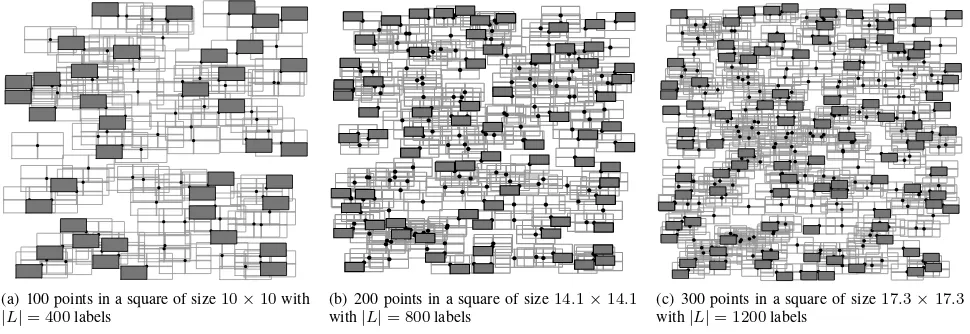
|L|/4], which implies on av-erage one point per unit area, and we generated four rectangular labels of width1and height0.5for each point, using the four position model. Afterwards, we slightly enlarged the rectangles, by offsetting their sides0.01units outwards. Due to this enlarge-ment, any two labels for the same point overlap. As a conse-quence, Constraint (4) is automatically satisfied in every solution without overlapping labels. Therefore, we did not instantiate that constraint in our tests. Figure 5 shows three instances that we generated this way.
To define the quality of a solution, we sampled the weightw(ℓ)
for each labelℓ∈Luniformly at random from the interval[0,1]. Furthermore, we definedρ= 0.02andα= 0.5. (Recall that we charge a cost ofα·w(ℓ)for any labeled point that is within dis-tanceρfrom a label of a different point.) Finally, to test the effect of Constraint (11), we defined that every axis-aligned square of size5×5must not overlap more thanKΓ= 10selected labels. Table 1 summarizes the results of our methods.
The first method, which we term ILP1, is based on an ILP using
• Constraint (3) to avoid overlapping labels,
• Constraint (6) to link thex-variables with they-variables,
• Constraint (11) to ensure that every axis-aligned square of size5×5overlaps at mostKΓ= 10labels, and
• Objective (7), which considers both weights of labels and costs for ambiguous label–point associations.
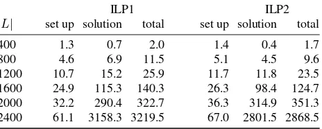
Table 1: Experimental results for instances with different num-bers but constant spatial density of rectangles: Number|L|of rectangles; average running times in seconds (for setting up and solving the ILP, and in total) with different ILP formulations. For each row, ten instances were tested.
ILP1 ILP2
|L| set up solution total set up solution total
400 1.3 0.7 2.0 1.4 0.4 1.7
800 4.6 6.9 11.5 5.1 4.5 9.6
1200 10.7 15.2 25.9 11.7 11.8 23.5
1600 24.9 115.3 140.3 26.3 98.4 124.7
2000 32.2 290.4 322.7 36.3 314.9 351.3
2400 61.1 3158.3 3219.5 67.0 2801.5 2868.5
For setting up ILP1 we need to find overlapping labels for Con-straint (3) and to compute the arrangement for ConCon-straint (11). This requires a considerable amount of time, which is shown in the second column of Table 1. For larger instances, however, the time for the set up of the ILP is clearly dominated by the time for the solution of the ILP, which is shown in the third column of Table 1. Solving an instance with 2400 labels requires almost one hour, which is certainly unacceptable in practice.
The second method, which we term ILP2, is very similar to ILP1. The only difference is that ILP2 does not use Constraint (6) to avoid overlapping labels. Instead, it uses Constraint (11) with
Γ = {(0,0)}and KΓ = 1. Recall that this means that ev-ery point in the plane is contained in at most one selected label, which is the same as forbidding label–label overlaps. As ILP1, ILP2 also uses Constraint (11) to avoid more than 10 labels in any square of size5×5, thus ILP2 uses Constraint (11) with two different settings forΓandKΓ, and it requires two arrangements to be computed. Therefore, the set-up time for ILP2 is generally higher than for ILP1. On the other hand, the solution time for ILP2 is usually lower, which can be explained with the fact that its LP relaxation yields a tighter upper bound for the objective value of an optimal ILP solution; see Sect. 2.5. Considering the total running times with ILP1 and ILP2, our experiments do not allow for a clear conclusion in favor of one or the other method. ILP2 seems to offer a small advantage, though.
4. CONCLUSION
We conclude that with our extended model we can effectively control the density of the labels in the output map and thus avoid situations in which the background map is occluded too much. Furthermore, our model improves the clarity of label–point as-sociations. If the input point set is not too dense, our ILP-based approach yields optimal solutions in reasonable time. With re-spect to cartographic quality, it would be interesting to see how our model extension performs with a more sophisticated weight function such as (Rylov and Reimer, 2014).
(a) 100 points in a square of size10×10with
|L|= 400labels
(b) 200 points in a square of size14.1×14.1 with|L|= 800labels
(c) 300 points in a square of size17.3×17.3 with|L|= 1200labels
Figure 5: Three instances with on average one point per unit area. Labels selected in an optimal solution are filled gray. Every axis-aligned square of size5×5overlaps at mostKΓ= 10selected labels.
References
Alinhac, G., 1962. Cartographie Th´eorique et Technique. Institut G´eographique National, Paris, chapter IV.
Been, K., Daiches, E. and Yap, C., 2006. Dynamic map labeling. IEEE Trans. Visual. Comput. Graphics 12(5), pp. 773–780.
de Berg, M., Cheong, O., van Kreveld, M. and Overmars, M., 2008. Computational Geometry: Algorithms and Applica-tions. 3rd edn, Springer TELOS, Santa Clara, CA, USA.
Doerschler, J. S. and Freeman, H., 1989. An expert system for dense-map name placement. In: Proc. Auto-Carto 9, pp. 215– 224.
Formann, M. and Wagner, F., 1991. A packing problem with applications to lettering of maps. In: Proc. 7th Annu. ACM Symp. Comput. Geom. (SoCG’91), pp. 281–288.
Imhof, E., 1975. Positioning names on maps. The American Cartographer 2(2), pp. 128–144.
Ribeiro, G. M. and Lorena, L. A. N., 2008. Lagrangean relax-ation with clusters for point-feature cartographic label place-ment problems. Comput. Oper. Res. 35(7), pp. 2129–2140.
Rylov, M. A. and Reimer, A. W., 2014. A comprehensive multi-criteria model for high cartographic quality point-feature label placement. Cartographica 49(1), pp. 52–68.
Verweij, B. and Aardal, K., 1999. An optimisation algorithm for maximum independent set with applications in map labelling. In: Proc. 7th Annu. European Symp. Algorithms (ESA’99), LNCS, Vol. 1643, Springer-Verlag, pp. 426–437.
Yoeli, P., 1972. The logic of automated map lettering. The Car-tographic Journal 9, pp. 99–108.
Zoraster, S., 1986. Integer programming applied to the map label placement problem. Cartographica 23(3), pp. 16–27.