OBJECT DEFORMATIONS FROM IMAGE SILHOUETTES USING A KINEMATIC
FINITE ELEMENT BEAM MODEL
C. Jepping*, T. Luhmann
Institute for Applied Photogrammetry and Geoinformatics (IAPG), Jade University of Applied Sciences Ofener Str. 16/19, 26121 Oldenburg, Germany - { christian.jepping, thomas.luhmann }@jade-hs.de
Commission V, WG V/1
KEY WORDS: Photogrammetry, silhouette, deformations, beam, finite elements
ABSTRACT:
In this paper a method is presented which allows the measurement of deflections and torsion by means of the silhouette of an object in images. The method is based on a finite element description of a beam. The benefit of this method is the determination of the deformation out of the silhouette of an object in images without the need of signalization.
The presented method is tested against simulated data as well as against real objects in laboratory tests.
As an outlook the presented method can be further modified. By combination with a laser scanner it seems to be possible to replace the CAD model of an object with the point clouds of one or more kinematic laser scans.
1. INTRODUCTION
In geodesy the measurement of deformations is a well-known topic. It ranges from measurement of discrete points up to surface comparisons with point clouds. Established methods like image matching or point tracking cannot be used for the registration of kinematic deformations of non-textured objects. One example is the measurement of rotor blade deformations on site. Due to the flexibility of the rotor blades themselves, the registration of deformations is a time-depending problem. By passing the tower of a wind power plant the rotor blades are affected by the air pressure close to the tower, for example. Additionally wind turbulences cause different deflections.
In principle one could signalize points, covering the whole surface, and apply photogrammetric multi-camera systems for measurement. With respect to a wind power plant this is a very expensive approach since the whole system has to be stopped (Sable, 1996), (Schmidt et al., 2009) and (Winstroth et al., 2014). Therefore a new photogrammetric target less approach has been developed using the silhouettes of the rotor blades in images. The method is based on a combination of image contour measurements with a kinematic finite element model of the object. Optionally points clouds of the surface, e.g. acquired by terrestrial laser scanning, or CAD models can be integrated.
2. PREVIOUS WORK
The following description of the previous work is separated in two parts: the first gives an overview of silhouette based methods and the second deals with modelling of deformations.
2.1 Silhouette-based photogrammetry
The silhouette (contour) is the outline of an object in an image. It is possible to estimate geometric primitives or poses by means of silhouettes. Andresen (1991) presented methods for fitting spheres or cylinders to the silhouette. Other examples of using silhouettes are given in Wong (2001). Potmesil (1986) describes a method for the calculation of the visual hull based on a set of
* Corresponding author
images. For the calculation of the visual hull an octree representation of the object space is used. For each element of the octree a visibility check is done. If a voxel lies inside the silhouette, it is part of the visual hull. Vice versa one can calculate the 6DoF parameters of a given object based on one image. Rosenhahn et al. (2004) use, among other approaches, a Fourier representation of the object geometry to calculate the pose of an object. Mokhtarian (1995) uses silhouettes for object recognition. In Cefalu & Boehm (2009) a method for recognition of objects based on a CAD representation of the object is presented. Combinations of 6DoF and deformation capturing are given in Rosenhahn & Klette (2004). They focus on human motion captured by cameras. The motion is calculated based on the silhouette of a person. To derive the motion information an initial model is set up which is deformed under the limitations of human motion.
2.2 Description of non-rigid deformations
Registration or tracking of non-rigid surfaces is investigated in different fields. Szeliskit & Lavallée (1993) are using deformable models for the registration of anatomical data, as an example. In robotics Fugl et al. (2012) apply a deformable object representation related to pick and place operations. In Jordt et al. (2015) an overview of different solutions is given.
These approaches could be distinguished in several ways. One is the kind of the representation of the deformation. Possible approaches are volumetric approaches which are widely used in matching of anatomical data or approaches based on the surface of an object. They use NURBS or mesh representations of a given model which is deformed by applying a deformation graph or function (Jordt & Koch, 2012; Li et al., 2009). With such a shape representation it is possible to determine the deformation of an object even out of only one image (Salzmann et al. 2007).
3. DESCRIPTION OF A NON-RIGID BEAM
As shown in section 2.2 there are different solutions for the description of a non-rigid object. The method presented in this
paper is based on a finite element description of a beam. In structural analysis a beam is a long and slender object, hence it is possible to model deflections and torsion of rotor blades by using a beam model description.
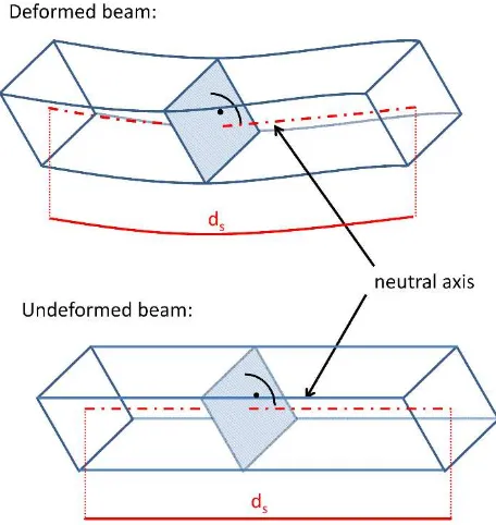
The used model is based on the assumptions of the Euler-Bernoulli beam theory: Firstly, a cross-section rectangular to the neutral axis remains rectangular to the deformed neutral axis, and secondly, a cross-section remains plain (Merkel & Öchsner, 2014). Furthermore it is assumed that a beam has the same length before and after a deformation.
Figure 1. Schematic of the assumptions of the deformations
3.1 A static non-rigid beam
To describe the deformation a so-called deformation graph is added to the object. In Li et al. (2009) the deformation graph describes the deformation of a 3D object. By using the assumptions of an Euler-Bernoulli beam this graph could be reduced to 1D. The CAD model of a beam-like object (e.g. a rotor blade) is divided into finite sections along the neutral axis. Between these sections transformation nodes Ki are defined, which are referenced to the neutral axis by their distances from the axis. The parameters of each node are describing six local transformations, namely three translations and three rotations. A given point of the CAD model PCAD is transformed by using the parameters of the neighbouring transformation nodes (Kl Kl+1). For the interpolation of the transformation parameters a base point PF is calculated, located on the neutral axis. The distances between this base point and the neighbouring transformation nodes act as weights in the interpolation process. (Figure 2).
The transformation equation of a point PCAD is given by:
F F CAD 0 0
CAD ( )
'
s P P P
R X
P = + ⋅ − +
s (1)
At this point the assumptions on the beam are still neglected. Without additional constrains the deformation can change the length of the deformed neutral axis in respect to the undeformed
neutral axis. Furthermore it is not given that a cross-section rectangular to the neutral axis remains rectangular after the deformation.
Figure 2. Schematic of point transformation
These assumptions can be considered by additional constraints (Jepping et al., 2016). Therefore three constrains have to be added for each transformation node, namely one for the distance between two nodes and two for the rectangular cross sections. As an alternative one can define the translation depending on the rotations. This has the advantage that the number of unknowns is reduced. Furthermore no constrains have to be added to the normal equation matrix.
For simplicity it is assumed that the neutral axis is a straight line along the x-axis of the beam coordinate system. Any deviation from this assumption can easily be described as a constant part of the deformation.
A rotation matrix can be defined as a set of three orthogonal and orthonormal vectors. The first vector is pointing in the direction of the rotated x-axis, the second intro the direction of the rotated y-axis and the third towards the rotated z-axis.
This definition is used to describe the deformation. Considering equation 1 we could rewrite the translation defined in a transformation node:
l
l K K
0 X' l X
X = − (2)
where
l K '
X are the coordinates of the deformed transformation
node and l K
X are the coordinates of the undeformed
transformation node. The coordinates of a transformation node at the index l can be expressed as:
x X =∆s⋅l⋅
l
K (3)
Where x is the vector {1;0;0}and ∆s is the distance between two nodes. Rewriting this equation yields:
x R X
0
Kl=∆s⋅l⋅ K (4)
It has to be noted that this equation is only valid in the undeformed case. In order to define the coordinates of a transformed transformation node the neutral axis is cut into pieces. Then the coordinates of a transformation node can be expressed by the coordinates of the previous transformation node, the previous rotation matrix and a constant distance between two nodes.
x R X
X
1 1
K
K − −
⋅ ∆ + =
l l
l s K (5)
Using this relation we can calculate the coordinates of every transformation node on the neutral axis. Furthermore the coordinates of the transformed base point Pf can be established
by means of the distance s of the base point on the x-axis.
On closer examination this definition shows some disadvantages. In equation 5 an interpolated rotation matrix is used for the transformation of a point. This means that a cross section does not remain rectangular to the neutral axis. To refine this approach the distances have to be scaled down. The result is the integral equation:
where R is an interpolated rotation matrix. The parameters ω, φ
and κ are interpolated along the neutral axis between RKl and RKl+1 by a linear interpolation. The interpolation function can be
written as:
Using equation 6 the translation in equation 1 can be described with the rotation matrixes defined in a transformation node. Using this description of a beam it is possible to model deflections and the torsion of a deformed beam.
3.2 A kinematic non-rigid beam
The transition from the static to the kinematic beam model can be achieved by adding the time to the transformation notes. As a consequence, the parameters ω, φ and κ have to be interpolated
over the distance s along the neutral axis and the time t. By using the bilinear interpolation the equation for the interpolation of ω
gives: transformation nodes. The first node has the indices K0,0. ∆s and
∆t are the steps in which the transformation nodes are defined over the distance and the time.
For solving the integral of equation 6 only the distance s is relevant. The new equation results to:
ds
regularizations are used. These regularizations are required in areas without observations. For a regular 2D grid Wendt (2008) proposed curvature minimizing functions. For the angle ω these are:The regularizations are added as observations with a particular weight. The weight is reduced depending on the actual iteration. In early iterations the weight is set to a high value. In the last iterations the weight is reduced. The goal of this process is that the raw deformation curves are estimated at first. In the last iterations the weight is reduced so that the effect of regularization affects only parts without or with few observations.
3.3 Global transformations
To separate the rigid from the non-rigid deformations a global transformation is added. One possible implementation is to define this transformation with the first transformation node by adding a translation. If a system of more than one beam is used this is not practicable. Furthermore the risk of a gimbal lock (Dam et al., 1998) by using Euler rotations for the transformations should not be ignored. For this reason the global transformation is defined as follow:
P R X
P'= + ⋅ (13)
In order to avoid the gimbal lock problem the rotations are defined by quaternions. The global transformation might be defined as static or as kinematic. In the following the kinematic definition is described. Similar to the non-rigid beam the transformations are defined at specified times. Between these times the parameters of the translation are interpolated linearly. For the quaternions it is not possible as simple as with the translations. By applying linear transformations between each parameter of a quaternion the resulting quaternion does not have to be a unit quaternion. Due to this reason a Spherical Linear Quaternion interpolation (Slerp) is used (Dam et al., 1998). In Slerp a quaternion is interpolated over the angle Ω between two quaternions q0 and q1:
One challenge using this equation is that the quaternion qt defines the same rotation as –qt. The angel between q0 and q1 can be different. Therefore the following definition is used:
If q0∙q1<0 than –q1 is used instead of q1. This causes an interpolation over the smaller angle.
Another problem is that equation 14 is not defined if q0 equals ±q1. In that case the interpolated quaternion equals q0 or q1.
3.4 Observations
As observations the image coordinates of the silhouette are used. These points are interpolated with subpixel accuracy. Between these points and the silhouette of the CAD model an Iterative Closest Point approach (ICP,Zhang, 1994) is applied.
To get the CAD model in image space each point of the model is transformed with the collinearity equations. From this 2D model the silhouette is extracted. In the extended ICP approach the deformations and the global transformations are estimated. To reduce the mismatches the gradients of the image points and the silhouettes are used. Only a point with similar gradient is
matched to a line of the silhouette. This is helpful for a slender object.
By using only photogrammetric observations the interpolation over time do not have to be applied if the transformation nodes are defined for each epoch. The interpolation becomes necessary if additional sensors such as laser scanners are used.
4. EXPERIMENTS
In this section two example experiments are presented. The first one is a test with synthetic images of rotor blades from a wind power plant. In this case a sequence of 10 seconds is simulated. The second one is a laboratory test. During this test a beam is oscillated and observed from two cameras and a multi camera system for reference.
4.1 Simulation
During the simulation a wind power plant is simulated with three rotor blades. Each of the rotor blades has a length of 60m. The rotor blade system is rotated and deformed over time. For the deformation each rotor blade is deformed separately. The deformation is described by two parabolas, one for the deflection in y- and one for z-direction. The parabolas have a minimum at the hub without deformation. The deformation at the tip of a rotor blade follows a periodic function. To keep the equidistance of the neutral axis the x-direction of the rotor blade is shortened
depending on the deformation in y- and z-direction. The torsion is described in a similar way.
Overall a maximum deflection of approximately 3m and a maximum torsion of approximately 5° are simulated.
The results of the simulation are three image sequences of three cameras (Figure3). In total each sequence has a duration of 10 seconds by 10 Hz. The cameras have a resolution of 1920x1440 pixels and a focal length of approximately 22mm. For more realistic results the images were affected by noise. The cameras were positioned in a triangle in front of the wind power plant. Two cameras are 90m away from the wind power plant and the second one 20m.
For the estimation of the deformation the beam model description of section 3.2 is used. The transformations nodes are defined in 7m steps along the neutral axis of the rotor blades with a time sequence of 0.1 seconds. For the global transformations a constant transformation is added for two of the three rotor blades (±120° rotations). Furthermore an unknown time depending global transformation is used (section 3.3).
For the calculation of the deformation an error-free CAD-model of the rotor blades is used. The exterior and interior camera parameters are error free, too.
To get start values for the calculation a 6DoF estimation is calculated at first. In this calculation the CAD model is used to calculate only the global transformation of each epoch. This is done separately for each epoch with start values based on the previous epoch.
Fig. 3: Example images of the sequence (top) and comparison between the determined (deformed) shape and the given shape from simulation after 2 sec and 4 sec (bottom)
length 60m
In a final step the deformations and the global transformations are estimated together. The result is a time depending description of the deformation and movements of the wind power plant. Based on these parameters deformed CAD models are exported. Comparisons are calculated with these models and the ground truth of the simulation.
The resulting deviations are only affected by the accuracy of the image measurement and the applied description of the deformation.
Therefore the results are too optimistic. In Figure 3 a comparison between the simulated ground truth and the calculated model at 2 seconds is shown. As could be seen, the deviations are very small. Overall the RMS of the comparison is 7mm. The maximum deviation is less than 30mm.
The high accuracy of the comparison is based on the error-free input data. In a real world example the accuracy will be lower. In further steps it is possible to use these results to identify critical components in the calculation of the deformation. As one example the influence of the CAD model as input data can be tested.
4.2 Laboratory test
In this test an oscillating aluminium beam is observed by two PCO DIMAX HD+ cameras with a resolution of 1920x1440 pixels. The cameras are used with a focal length of approximate 22mm. The image scale is approximately 1:24. The aim of the test is the measurement of the kinematic deformation of the beam by using the silhouette of the beam in images. For a reference measurement circular targets are used. These targets are observed by the same cameras as used by the silhouette approach. As a result there is no additional transformation required between the reference system and the measuring system. The test set up is shown in Figure 4.
The oscillation is captured with 50Hz. For the calculation the transformation nodes are defined each 5cm with a time sequence of 1/50 seconds. To show the ability of the method the coordinate centre of the global transformation is set to the tip of the beam. To get a more stable global transformation a transverse beam was glued to the main beam (Figure 4). This case is a more realistic setup than a fixed coordinate system at the mounted side of the beam.
Because of the uncertainty of the glued beam the relative rotation between the main beam and the glued beam is set as unknown and constant for each epoch.
The result of the calculation is promising. In the comparison the distances between the measured points and the calculated deformed model are calculated. Figure 5 shows a comparison for one epoch.
The maximum deviation to the reference is 0.5mm with an RMS value of 0.15mm. As could be seen in Figure 5 the deviations between reference and the silhouette approach are much higher at the shorter beam than at the long one. The maximum deviation on the long beam is 0.08mm caused by the set up. The main deformations of the shorter beam are in the line of sight of the cameras. The viewing angles between the longer beam and the cameras are much better.
The standard deviation of the reference is approximately 0.02mm. This leads to the conclusion that the reference is not accurate enough in the case of the long beam.
For a more detailed analysis the standard deviations of a transformed point of the CAD model are calculated (deformation and global transformation). For a point close to the transformation node at 400mm the standard deviation is approximately 0.04mm. This matches to the reference measurements. At the short beam the standard deviation is much higher. It rises up to 0.12mm.
For a detailed analysis the correlation between the global transformation and the deformation is calculated. The parameters are very high correlated with the global transformation of to 0.75. That means that a deformation is not clearly separable from the global transformation. In the case of this experiment it is easy to define the global transformation into the fixed end of the beam. That would result in a reduction of the correlation between the deformation and the global transformation. But that is not possible in the case of a rotor blade.
Figure 4. Laboratory set up
A more realistic way is the use of additional information like a CAD model from a nacelle in the case of rotor blades or the behaviour of the object. In the case of a beam the bending stiffness is a possible criteria. In this example the stiffness in the y-direction is much higher than in the z-direction of the beam. Using a higher weight for the regularization in the y-direction leads to a reduction of the standard deviation in the y-direction.
5. EXTENSIONS AND OUTLOOK
The presented method could easily be extended in several ways. One extension is an adaptive weight for the regularizations depending on the characteristics of the object. One example is the stiffness of a rotor blade. The stiffness is much higher at the hub then at the tip of a rotor blade. In this case it makes sense to define a high weight for the regularization at the hub and a lower at the tip of the rotor blade. Another extension is the use of contour lines or well defined points at the object. An example of a well-defined contour line is the trailing edge of a rotor blade. This could be extracted using methods like the LSB-snakes (Gruen & Li, 1997). A promising extension is the use of additional sensors like laser scanners. Laser scanner point clouds are already supported and are advantageous for the calculation of the torsion angle. The point cloud is used in an extended ICP approach. The distances between the time depending object and the measured points are minimized.
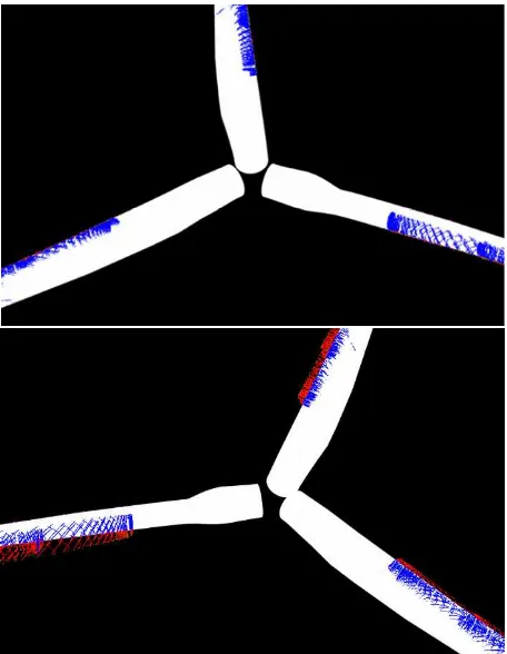
To get rid of the CAD model it seems to be possible to combine lasers scanner point clouds and photogrammetry. Instead of the CAD model the 3D profiles are used. Figure 6 shows two steps in the calculation.
In a first step the rotation of the rotor blade system is determined from the images. After this step it is possible to transform the laser scanner points into the coordinate system of the rotor blades (Figure 6 bottom). For a more accurate transformation the deflection can be determined by the use of the trailing edge in images. In a final step the distances between selected points from
the point cloud in image space and the silhouette of the rotor blade in images are minimized. The result is shown in Figure 6 top.
The main problem in the calculation of the deformation without a CAD model is the identification of possible matches between the silhouette in images and the laser scanner points. Especially at the tip of a rotor blade an identification of possible matches is a problem. A possible match is defined by using the distances between the points of a measured profile and the silhouette. For the identification of possible matches a few constrains have to be respected. The first and last points of a profile are no possible matches. A possible match has to be a local extreme value. For this analysis a signed distance is required. Points outside the silhouette have a negative distance and points in the inside of the silhouette have a positive distance to the corners of the silhouette. Due to these constrains there are restrictions for the position of the laser scanner due to the cameras and the object. Furthermore there are restrictions on the observed object, too.
Figure 5. comparison between the determined (deformed) shape and the targeted points on the beam
Figure 6. Visualisation of the matching between laser scanner profiles and silhouette. Red points are outside the silhouette and
blue points are inside. The final result is shown in the top image. An overlay with start values is shown in the bottom
image.
6. SUMMARY
In this publication a method is described which allows the determination of deflections and torsion out of the silhouette in images. This method was tested against simulated data and laboratory tests. In these tests the benefit and the limitations of the method could be shown. Especially the laboratory test shows the dependency on a good setup. Deflections in the direction of the line of sight are less accurate than other ones.
Furthermore a high correlation between the deformation and the global transformation could be observed. These correlation leads to the conclusion that the deformation could only be observed with a high accuracy if the global transformation of the beam is accurate. One proposal for the reduction of the correlation is to use as much preliminary information as possible.
Furthermore, possible extensions have been discussed. One of these extensions is the combination of laser scanning and photogrammetry.
REFERENCES
Andresen, K. 1991. Ermittlung von Raumelementen aus Kanten im Bild. Zeitschrift für Photogrammetrie und Fernerkundung, 59(6), 212-220.
Cefalu, A., Boehm, J. 2009. Three-dimensional object recognition using a monoscopic camera system and CAD geometry information. SPIE Optical Engineering+ Applications (). International Society for Optics and Photonics, pp. 74470K-74470K
Dam, E. B., Koch, M., Lillholm, M. 1998. Quaternions, interpolation and animation. Datalogisk Institut, Københavns Universitet.
Große-Schwiep, M., Piechel, J., Luhmann, T. 2013. Measurement of Rotor Blade Deformations of Wind Energy Converters with Laser Scanners. ISPRS Annals of the Photogrammetry, Remote Sensing and Spatial Information
Sciences, Volume II-5/W2, ISPRS Workshop Laser Scanning
2013, Antalya, Turkey.
Gruen, A., Li, H. 1997. Semi-automatic linear feature extraction by dynamic programming and LSB-snakes. Photogrammetric
Engineering and Remote Sensing, 63(8), pp. 985-994.
Jepping, C., Schulz, J. U., Luhmann, T. 2016. Konzept zur Modellierung kinematischer Rotorblattverformungen an Windkraftanlagen. Allgemeine Vermessungsnachrichten, 1, pp. 3-10.
Jordt, A, Koch, R 2012. Direct Model-based Tracking of 3D Object Deformations in Depth and Color Video, International
journal of computer vision, 102(1-3), pp. 239-255.
Jordt, A., Reinhold, S., Koch, R 2015. Tracking of Object Deformations in Color and Depth Video: Deformation Models and Applications, Proc. SPIE 9528, Videometrics, Range Imaging, and Applications XIII
Li, H., Adams, B., Guibas, L. J., Pauly, M. 2009. Robust single-view geometry and motion reconstruction. In ACM Transactions on Graphics (TOG) (Vol. 28, No. 5, p. 175). ACM.
Merkel, M., Öchsner, A. 2014. Eindimensionale finite Elemente:
ein Einstieg in die Methode. 2. Auflage, Springer Verlag, Berlin.
Özbek, M. 2013. Optical monitoring and operational modal analysis of large wind turbines, Dissertation, Delft University of Technology.
Potmesil, M. 1987. Generating octree models of 3d objects from their silhouettes in a sequence of images, CVGIP 40, pp. 1–29.
Rosenhahn, B. and Klette, R., 2004. Geometric Algebra for Pose Estimation and Surface Morphing in Human Motion Estimation, Combinatorial Image Analysis. Springer Berlin Heidelberg, 2004. Pp. 583-596.
Rosenhahn, B., Sommer, G., Klette, R. 2004. Pose Estimation of Free-form Objects (Theory and Experiments). Bericht Nr. 0401, Christian-Albrechts-Universität, Kiel.
Sabel, J. C. 1996. Optical 3D motion measurement. In Instrumentation and Measurement Technology Conference, 1996. IMTC-96, Conference Proceedings, Quality
Measurements: The Indispensable Bridge between Theory and Reality, IEEE (Vol. 1, pp. 367-370).
Salzmann, M., Pilet, J., Ilic, S., Fua, P. 2007. Surface deformation models for non-rigid 3D shape recovery. Pattern Analysis and
Machine Intelligence, IEEE Transactions on, 29(8), pp.
1481-1487.
Schmidt Paulsen, U., Erne O., Schmidt, T. 2009. Wind Turbine Operational and Emergency Stop Measurements Using Point Tracking Videogrammetry, Proceedings of the SEM Annual Conference, Albuquerque, New Mexico, USA.
Szeliski, R., Lavallee, S. 1993. Matching 3D anatomical surfaces with nonrigid deformations using octree splines. In SPIE's 1993 International Symposium on Optics, Imaging, and Instrumentation. International Society for Optics and Photonics, pp. 306-315
Wendt, A. 2008. Objektraumbasierte simultane multisensorale Orientierung. Dissertation, Fakultät für Bauingenieurwesen und Geodäsie, Leibniz Universität Hannover. Wissenschaftliche Arbeiten der Fachrichtung Geodäsie und Geoinformatik der Leibniz Universität Hannover, ISSN 0174-1454
Winstroth, J., Schoen, L., Ernst, B., Seume1, J. R. 2014. Wind turbine rotor blade monitoring using digital image correlation: a comparison to aeroelastic simulations of a multi-megawatt wind turbine, Journal of Physics: Conference Series 524 (2014) 012064
Wong, K. Y. 2001. Structure and motion from silhouettes. Dissertation, University of Cambridge, Cambridge.
Zhang, Z. 1994. Iterative point matching for registration of free-form curves and surfaces. International Journal of Computer Vision, 13(2), 119-152.