A HYBRID APPROACH TO EXTRACTION AND REFINEMENT OF BUILDING
FOOTPRINTS FROM AIRBORNE LIDAR DATA
Hai Huang*, Monika Sester
Institute of Cartography and Geoinformatics, Leibniz Universität Hannover, Appelstr. 9a, D-30167 Hannover,
Germany
{Hai.Huang, Monika.Sester}@ikg.uni-hannover.de
Commission IV, WG IV/4
KEY WORDS: Urban, Building, Extraction, LIDAR, Point Cloud, Three-dimensional
ABSTRACT:
This work presents a combined bottom-up and top-down approach to extraction and refinement of building footprints from airborne LIDAR data. Building footprints are interesting for many applications in urban planning. The cadastral maps, however, may be limited for certain areas or not be updated frequently. Airborne laser scanning data is therefore considered by many people in the last decade as an important alternative data for change detection and update of building footprints. Laser scanning data of city scenes, however, often shows noise and incompleteness because of, e.g., the clutter by vegetation and the reflection of windows/waterlogged depressions on the roof. Results of the bottom-up detection may thus be limited to incomplete or irregular polygons. We employ 3D Hough transform to detect the building points. An improved joint multiple-plane detection scheme is proposed to find and label the laser points on multiple roof facets synchronously. The bottom-up processing provides not only a rough point segmentation but also additional 3D information, e.g., roof heights and horizontal ridges. Using these as priors, a top-down reconstruction is conducted via generative models. We consider the building footprint as an assembly of regular primitives. A statistical search by means of Reversible Jump Markov Chain Monte Carlo and Maximum A Posteriori estimation is implemented to find the optimal configuration of the footprint. By these means a robust and plausible reconstruction is guaranteed. First results on point clouds with various resolutions show the potential of this approach.
* Corresponding author.
1. INTRODUCTION
In the past decades many approaches for the extraction and reconstruction of building models from measurement data have been reported. The data sources include aerial and satellite photographs, synthetic aperture radar (SAR) images, and airborne and terrestrial laser scanning data. Overviews are given by Brenner (2005), Schnabel et al. (2008), and Vosselman (2009). Additionally, digital surface models (DSMs) generated by interpolation from laser point clouds or stereo-pair-images are used as the basis for the reconstruction of building outlines (Ortner, 2007) and 3D buildings (Lafarge, 2010).
Building footprints are interesting for many applications in urban planning. The cadastral maps, however, may be limited for certain areas or not be updated frequently. Airborne laser scanning data is therefore considered by many people in the last decade as an important alternative data for change detection and update of building footprints. In (Pfeifer et al., 2007), an overview of the algorithms and methods of quality assessment are given. Recent works include (Lafarge et al., 2008), in which building footprints are modeled as connected rectangles and detected based on marked point processes from DSM, and (Rutzinger et al., 2010), which focuses on the large scale building change detection from airborne laser scanning data.
Building detection is often based on the extraction of planar surfaces. 3D Hough transform (Vosselman and Dijkman, 2001) is an application of the 2D Hough transform technique (Hough, 1962). In the context of laser scanning, it is often employed for
plane detection. One plane in object space can be mapped to a point in parameter space and then the mapping of all possible planes passing through the point in object space leads to a certain manifold in parameter space. The coplanar condition of multiple points can therefore be equally expressed as the intersection of their corresponding manifolds. Recently, this technique has been extended in (Rabbani and Van den Heuvel, 2005) to detect more complicated geometries, e.g., cylinders.
Airborne laser scanning data of city scenes, however, often shows noise and incompleteness because of, e.g., the clutter by vegetation and the reflection of windows and waterlogged depressions on the roof. Direct results of the bottom-up detection may thus be limited to incomplete or irregular polygons.
This paper presents a hybrid approach to extraction and reconstruction of building footprints from airborne laser scanning data combining bottom-up roof plane detection and top-down footprint reconstruction via generative models. We show how additional 3D information improves the 2D footprint reconstruction. We employ 3D Hough transform to detect the building points. Following (Huang and Brenner 2011), an improved joint multiple-plane detection scheme is proposed to find the roof facets, as well as the laser points belonging to the same building synchronously. A generative statistical approach is then conducted for the footprint reconstruction. We consider the building footprint as an assembly of regular primitives, which are parameterized in a predefined library. Based on an initial model provided by the bottom up process a search by International Archives of the Photogrammetry, Remote Sensing and Spatial Information Sciences, Volume XXXVIII-4/W25, 2011
means of Reversible Jump Markov Chain Monte Carlo (RJMCMC) and Maximum A Posteriori (MAP) estimation is implemented to find the optimal reconstruction.
The next sections are organized as follows. Section 2 introduces 3D Hough transform and the multiple-plane detection scheme. A primitive-based generative statistical modeling is described in Section 3. Section 4 presents the optimization with MAP estimation. First experiment results shown in Section 5 demonstrate the potential of the proposed approach. The paper ends up with conclusion and outlook.
2. PLANE DETECTION
Planes are often the basis of building detection and can be obtained employing various algorithms. The mostly used techniques for plane detection from point clouds include Hough transform, Region Growing, and Random Sample Consensus (RANSAC). No matter which technique is chosen, they share a similar scheme: first finding one plane each time, then removing the corresponding points, and going on with the next one in the next iteration. The possible problems are: (1) time consuming search as the remaining points are calculated repeatedly until they have been recognized and removed; (2) points that belong to two adjacent planes may be too early removed with the firstly found plane. To avoid these drawbacks we propose a joint plane detection scheme by enhancing the Hough transform to find multiple planes synchronously. By this means the points are used more efficiently – they are calculated for only one time while being allowed to vote multiple planes.
The basic purpose of the plane detection is to find and label data points on the roof implying a rough outline (2D) of the target building. Since the planes are actually found in 3D, additional instructive information: roof heights and horizontal ridges (of hipped roofs) can be derived from the available plane parameters and used to guide the further reconstruction.
2.1 Pre-segmentation
Dealing with relatively large scenes, in which multiple buildings or building groups exist, a pre-segmentation provides the following advantages:
1. The result of 3D Hough transform becomes more stable with limited numbers of points as well as underlying planes.
2. The MCMC search is conducted locally, i.e., the sampler does not need to travel the whole scene overcoming many local minima to find the target, which guarantees the efficiency and convergence.
Figure 1. Pre-segmentation: the given point cloud (left) is converted into a raster image (middle). After morphology processing blobs containing individual buildings are labeled and segmented (red dashed rectangle).
As shown in Figure 1 the point cloud of a test zone (left) is converted into a grayscale image (middle) with the gray value of each pixel indicating the elevation. Buildings, as well as a number of other objects, mostly trees, are presented as brighter areas with higher elevation over the ground. We employ mathematical morphology to reduce small spots, which suppose to be non-building objects. Let I be the input image and s the structuring element, which is defined as a disk with a radius of 5 meters, an “Opening” operation
is conducted with “Erosion” and subsequent “Dilation”. Essential effects of “Opening” are to remove the trivial spots and restore the outline. The relatively large “blobs”, which are supposed to contain individual buildings or building groups, are thereby clearly separated in spite of the numerous adjacent noises and shown in a binary image (Figure 1, middle).
The point cloud is segmented into subzones based on the detected blobs. A subzone is defined as the minimum circumscribed rectangle (or “bounding box”, cf. Figure 1, right, red dashed rectangle) of the blob and a few more meters tolerance is given according to the size of the employed structuring element.
Plane detection and footprint reconstruction are conducted in individual subzones with reduced calculation complexity. The subzones have a local coordinate system for calculation and keep the original (global) coordinates as well. The latter is used to reconstruct the complete scene by assembling the individual footprints.
2.2 3D Hough Transform
3D Hough transform is chosen as basis for the proposed plane detection because of its potential of finding multiple planes synchronously.
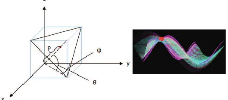
As shown in Figure 2 (left), the polar coordinates of the plane are employed as its parameters. A plane passing through the point (x, y, z, Cartesian-coordinates) can then be expressed as
θ θ ϕ θ ϕ
ρ=xcos cos +ysin cos +zsin (1)
with φ the azimuth, θ the angle of elevation, and ρ the normal distance from the origin to the plane. We define the origin to be lower than the whole point cloud so that the ranges of φ and θ can be reduced to φϵ [0°, 180°] and θϵ [0°, 180°], i.e., only the upper half-sphere.
Figure 2. Definition of the Cartesian- and polar-coordinates for the transform (left) and a 3D view of Hough space (right). 3 manifolds intersect at one point (red circle) in Hough space indicates 3 points defining one plane in Euclidean space. International Archives of the Photogrammetry, Remote Sensing and Spatial Information Sciences, Volume XXXVIII-4/W25, 2011
The plane is presented as a point in its parameter space – Hough space. All possible planes passing a single point then form a manifold in Hough space. As shown in Figure 2 (right), 3 manifolds intersect at one point (red circle), which is corresponding to 3 points determining one plane in Euclidean space. Theoretically, if there are n (n ≥ 3) coplanar points in object space, an exclusive intersection position of their corresponding manifolds should exist in Hough space as well. In practice, however, they may not perfectly meet at one point because of the noise. On the other side, there are many trivial intersections as an arbitrary non-colinear point-triplet determines a plane. To find the best estimation of the common plane we, therefore, look for the position, where the manifolds show the highest degree of concentration rather than chasing the intersected locations. Mapping only the maximum concentration degree for each φ-θ location, the Hough space can be plotted into 2D, as shown in Figure 3.
Figure 3. 2D plots (azimuth-elevation) of 3D Hough spaces for 4 points voting 1 plane (left), 120 points/3 planes (middle) and the test zone (4800 points/6 planes, right). A lighter pixel indicates a higher manifolds concentration.
According to the density and quality of the point cloud a threshold can be set (manually) to accept all the potential planes. Yet, as the number of points increases, the results no more concentrate well (cf. Figure3, middle and right). This is particularly crucial for non-flat roofs. A post-processing is needed to analyze the results.
2.3 Joint Plane Detection
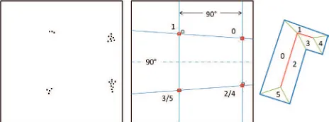
As shown in Figure 4, a joint multiple-plane detection scheme is employed to find plausible construction from the fuzzy results. The sketch in φ-θ diagram (left) demonstrates a filtered result of the 3D Hough transform. Although the top candidates of φ-θ are well concentrated in four groups, simple clustering and averaging of them still lead to obvious errors (middle, gray rectangles). Assuming these planes belong to an individual building, basic constraints can be derived without knowing the actual configuration:
– Planes sharing a horizontal ridge have the same azimuth. E.g., for planes 0 and 2 (cf. Figure 4, right): if |φ0−φ2| < 5° or > 175°, then adjust |φ0−φ2| = 0° or 180°. The variation of each φ is inversely proportional to the number of the coplanar points.
– Planes sharing a horizontal ridge follow θ0+θ 2 = 180° if |φ0−φ2| = 0° or θ0 = θ2 if |φ0−φ2| = 180°, which implies that the roof has a symmetrical form.
– Planes sharing a diagonal ridge have perpendicular azimuths. E.g., for planes 0 and 1: if |φ0−φ1| ϵ (90°±5°), then force |φ0−φ1| = 90°.
These rules work only based on the parameter values while the context (adjacency) relation of the planes is still unknown. The result is thereby refined as shown in Figure 4 (middle, red rectangles). Please note that this diagram only shows the
distribution on azimuth-elevation, i.e., parallel planes are shown at the same position (cf. positions 3/5 and 2/4). They, however, can be easily separated by their different ρ values. Figure 5 (middle) presents the detected planes by labeling the coplanar points with different colors.
Figure 4. Joint adjustment of plane parameters: the preliminary result of the 3D Hough transform (left), results before (gray) and after (red) joint planes adjustment (middle), and the underlying model (right)
The advantages of the proposed scheme are:
1. The parameters of multiple planes are jointly adjusted, i.e., points of multiple planes contribute to their common parameter, e.g., azimuth of planes 0 and 2, making the result more accurate and reasonable.
2. No point-deletion during the detection. Points in adjacent areas are allowed to vote multiple planes instead of being removed too early with the first found facet. The point cloud can thus be used more efficiently leading to more robust detection.
2.4 Initial Contour and Additional 3D Information
We note that simple morphology processing already provide some meaningful contours, which in many cases can even be directly used for footprint reconstruction. The more expensive 3D plane detection is implemented because it can sort out non-planar objects, i.e., trees (cf. Figure 1, right, green dashed outlines) as well as provides instructive 3D information. The following information can be derived from the plane detection (cf. Figure 5):
1. Roof points: the data points that belong to the roof planes are labeled, implying a rough outline (blue dashed line) of the target building.
2. Roof Heights: different roof heights indicating separate building parts.
3. Ridges (non-flat roofs): horizontal ridges (red lines) and diagonal ridges (green lines) are calculated by intersecting planes.
Figure 5. The output of the bottom-up process: the point cloud (left), the roof points (middle) labeled with colors indicating a rough building outline (blue dashed contour), and horizontal (red lines) as well as diagonal (green lines) ridges (right) International Archives of the Photogrammetry, Remote Sensing and Spatial Information Sciences, Volume XXXVIII-4/W25, 2011
Although the ridges are not shown in the building footprint, they provide essential constraints for the reconstruction. Especially, horizontal ridge is the key as it mostly indicates the main axis of the building. Please note, although the plane detection and the building outline can be rough, the determination of ridges has higher accuracy as their parameters can be seen as a synthesis of all the related planes’ parameters.
3. HYPOTHESES GENERATION
In the generative reconstruction, a building footprint is considered as a variant of a single primitive or an assembly of multiple primitives. One or more primitives are instantiated and fitted into the point cloud, until the majority of the points are represented by the primitives. The main advantage of the generative reconstruction is the guarantee of plausible results. The influence of the clutter by vegetation and errors in the point cloud may be significantly reduced.
A statistical search is conducted by means of Reversible Jump Markov Chain Monte Carlo. The initial information derived from plane detection (cf. Section 2.4) is integrated into the search in the form of priors.
3.1 Primitive-based Modeling
We use square and rectangle as the primitives of footprints. The rectangle has 5 parameters: length (l), width (d), azimuth (α), coordinates of the centroid (x, y) while the square has 4 (l=d). Through sampling the parameters a large number of hypothesis models are generated and the best candidate is found in the optimization (cf. Section 4).
Being different from most approaches, overlapping is allowed in the combination of primitives. By this means (1) a number of complex buildings are possible to be represented by simple primitives and (2) the primitives can maintain the regularity during the reconstruction instead of being cropped into irregular facets to fit the data. The side effect – the redundant parts are always hidden inside the assembly and they can be easily removed by “merging” the primitives with usual geometrical tools.
3.2 Priors
As mentioned before, horizontal ridge is the key of the roof geometry. Knowing it as y=ax+b|hridge, constraints can be derived for the footprint parameters.
1. The horizontal ridge indicates the orientation of the primitive: 2. Projection of the horizontal ridge is very likely in the axis of the primitive. The centroid of the primitive is located on it. x and y are then coupled as:
with b the y-intercept. The normal deviation of the footprint central axis to the horizontal ridge is allowed and can be calculated as ∆=cosα∙|bcentroid - bhridge| for asymmetry roofs.
The sampling of parameter space Θ={x, y, α, l, d} is now
equivalent to the sampling of Θ’={x, α, b, l, d}. Although the
size of Θ is the same, the parameters that have large searching ranges are now narrowed down to {x, l, d} as the standard deviations for α and b are mostly very small. Furthermore, the number of horizontal ridges also implies the minimum number of primitives, which gives prior information for the Reversible Jumps (cf. Section 3.3).
Priors for l and d can be derived from the initial building outline. The search space of parameters is thereby significantly reduced making the sampling faster and more stable.
3.3 Statistical Sampling
Reversible Jump MCMC is an extension of the MCMC algorithm to handle variable-dimension solution spaces. As proposed in (Green, 1995), the Markov Chain sampler is allowed to switch between subspaces with variable dimensions in the search. The dimension jumps, i.e., modeling with varying numbers of parameters or/and objects, is employed in this work to simulate the choice of different configurations of primitives.
RJMCMC has a mixed transition kernel, which defines all possible movements:
– Sw1: “switch” to primitive with n+1 parameters
(square to rectangle);
– Sw2: “switch” to primitive with n−1 parameters
(rectangle to square);
– Bi: “birth” of a new primitive adjacent to the existing one;
– De: “death” of the last born primitive.
Let Mi and Mj be states (configurations) before and after a
movement. The “detailed balance” condition in the Markov Chain can be expressed as:
j
The Markov Chain is constructed with Metropolis-Hastings algorithm as:
The RJMCMC sampling can be summarized as follows:
1. Initialization: (M(i=0), Θ(i=0)) 2. Proposing new state M’
2.1 sampling configuration from {u, Sw1, Sw2, Bi, De} with u ~ U [0,1]
2.2 sampling parameters Θ’
3. Accepting new proposal with probability
Please note that as long as the jump kernels keep the balance condition, i.e., being reversible – possible to return to the pre-vious state, the RJMCMC sampler can explore in a great wider variety of hypothesis models. This makes RJMCMC itself has a powerful “model selection” effect, i.e., the ability to find opti-mal configuration of the model.
4. LIKELIHOOD AND OPTIMIZATION
4.1 Likelihood Function
We define the quality of footprint reconstruction as follows and use it for the likelihood of hypotheses:
(
)
reconstructionTP
– TP: True Positive, building points that have been included inside the footprint;
– FP: False Positive, building points outside the footprint;
– FN: False Negative, the included positions (for raster data only) has no building points.
4.2 Optimization
In the random search, sometimes, incorrect parameters may lead to same or even better score for reconstruction because of the clutter and flaw in the data. To deal with this we employ the posterior instead of the likelihood of the proposal M (with parameter space Θ) as the goal function in the optimization:
(
) (
and can be seen as a constant in the optimization. The MAP estimation of Θ can then be expressed as:As shown in Equation 12, additional to the likelihood of the
reconstruction the plausibility of individual parameters is also taken into account in the optimization. Multiplication is used to integrate the priors making sure that unreasonable hypotheses will have much lower posterior and can be more easily recognized.
5. EXPERIMENTS AND DISCUSSION
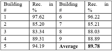
First experiment is conducted for an urban scene with the data point density of 1 meter. Figure 6 shows in red the primitives
(left), which the buildings consists of. In blue, the primitives are merged into result footprints (middle) and the ground plan is given in green (right). The assessment of the reconstruction is given in Table 1.
Figure 6. Footprint reconstruction of a scene with multiple buildings: the extracted primitives (left), reconst-ructed footprints (middle), and the ground truth data (right) from cadastral map as reference
Building
Table 1: Assessment of the footprints reconstruction
The problems in the reconstruction of building 3 (cf. Figure 7) can be explained as follows: first of all, in the north part there are two low roofs, which were not reconstructed by our method, since their height is lower than the search range. Secondly, there are small extrusions to the left and the right of the building, which could not be reconstructed because they are not represented by enough LIDAR points. This explains also the obvious deviation for building 7 (with a lower terrace) and some missing narrow and small parts.
Figure 7. Building parts with lower roofs and smaller extrusions have not been reconstructed: footprint in point cloud (left), compaison with given ground plan (middle), and an aerial image as reference (right)
High resolution data, relatively speaking, is able to provide higher accuracy and represent small structures more meaningfully. As shown in Figure 8, superstructure, in this case a chimney (black), has been extracted from a point cloud with the density of about 0.18 meter. A more detailed footprint (blue) is reconstructed including the chimney shaft. Without ground truth data, the result is projected (red contour) into the raster image (right) of the data for comparison. Please note the lighter margin outside the red contour approximately indicates the protrusion of the roof, which has been recognized as the ground points below are also available.
Figure 8. More detailed footprint is reconstructed from the point cloud with high density.
6. CONCLUSION AND OUTLOOK
This paper presents a hybrid approach to building footprint extraction and reconstruction from airborne laser scanning data. The main contributions can be summarized as follows:
– Point cloud segmentation based on 3D plane detection, from which additional 3D geometrical information is extracted and utilized to improve the 2D footprint reconstruction;
– Primitive-based modeling of building footprints allowing overlapping;
– A generative statistical reconstruction driven by RJMCMC.
By these means a robust and plausible reconstruction of building footprints is ensured.
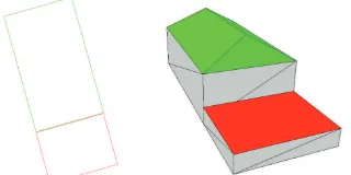
Please note in Figure 6, building 9 is reconstructed with two adjacent parts instead of one block because the roof planes has been found with very different heights and treated as separate building parts (Figure 9, left). On this basis, the same top-down reconstruction can also be considered for the enrichment of existing ground plans by 3D-information in terms of LoD 1 and LoD 2. To this end, a given ground plan, possibly consisting of different roof types, can be reconstructed as shown in Figure 9 (right). A work towards this can be found in (Huang et al. 2011).
Figure 9. Enrichment of cadastral maps with different roof heights and types
In this work only simple square and rectangle are used as primitives. A majority of the buildings can be represented or approximated by them. The primitive library, nevertheless, can be easily extended with triangle, circle and ellipse to present more sophisticated buildings like exhibition centers and stadia.
REFERENCES
Brenner, C., 2005. Building reconstruction from images and laser scanning. International Journal of Applied Earth Observation and Geoinformation, Theme Issue on Data Quality in Earth Observation Techniques, 6(3-4), pp. 187–198.
Green, P., 1995. Reversible Jump Markov Chain Monte Carlo Computation and Bayesian Model Determination. Biometrika, 82:711-732.
Hough, P., 1962. Method and means for recognizing complex patterns, U.S. Patent 3,069,654.
Huang, H. and Brenner, C., 2011. Rule-based roof plane detection and segmentation from laser point clouds. In: Joint
Urban Remote Sensing Event (JURSE) 2011, pp. 293–296.
Huang, H., Brenner, C. and Sester, M., 2011. 3D building roof reconstruction from point clouds via generative models. In:
ACM SIGSPATIAL, the 19th
International Conference on Advances in Geographic Information Systems, (submitted).
Lafarge, F., Descombes, X., Zerubia, J. and Pierrot-Deseilligny, M., 2008. Automatic building extraction from DEMs using an object approach and application to the 3d-city modeling. ISPRS
Journal of Photogrammetry and Remote Sensing, 63(3), pp.
365–381.
Lafarge, F., Descombes, X., Zerubia, J. and Pierrot-Deseilligny, M., 2010. Structural approach for building reconstruction from a single DSM. IEEE Transactions on Pattern Analysis and Machine Intelligence, 32, 135–147.
Ortner, M., Descombes, X., and Zerubia, J., 2007. Building outline extraction from digital elevation models using marked point processes. International Journal of Computer Vision, 72(2), pp. 107–132.
Pfeifer, N., Rutzinger, M., Rottensteiner, F., Muecke, W. and Hollaus, M., 2007. Extraction of building footprints from airborne laser scanning: Comparison and validation techniques. In: Urban Remote Sensing Joint Event, pp. 1–9.
Rabbani, T. and Van den Heuvel, F., 2005. Efficient Hough transform for automatic detection of cylinders in point clouds.
In: ISPRS Workshop Laser Scanning, Enschede, the
Netherlands.
Rutzinger, M., Rüf, B., Vetter, M., and Höfle, B., 2010. Change detection of building footprints from airborne laser scanning acquired in short time intervals. In: The International Archives of Photogrammetry, Remote Sensing and Spatial Information Sciences, 38(7B), pp. 475–480.
Schnabel, R., Wessel, R., Wahl, R. and Klein, R., 2008. Shape recognition in 3d point-clouds. In: The 16th International Conference in Central Europe on Computer Graphics, Visualization and Computer Vision.
Vosselman, G., 2009. Advanced point cloud processing. In:
Photogrammetric Week ’09, pp. 137–146.
Vosselman, G. and Dijkman, S., 2001. 3D building model reconstruction from point clouds and ground plans. In: The International Archives of the Photogrammetry, Remote Sensing and Spatial Information Sciences, 34(3/W4), pp. 37–43.
ACKNOWLEDGEMENTS
We thank Deutsche Forschungsgemeinschaft (DFG) for supporting Hai Huang under grant BR2970/2-2.