VEGETATION CHARACTERISTICS USING MULTI-RETURN TERRESTRIAL LASER
SCANNER
Francesco Pirottia,*, Alberto Guarnieria, Antonio Vettorea a
CIRGEO-Interdepartmental Research Center for Geomatics, University of Padova, viale dell'Università 16, 35020 Legnaro Padova, Italy (francesco.pirotti, antonio.vettore, alberto.guarnieri)@unipd.it
Commission V, WG V/3
KEY WORDS: terrestrial laser scanning, vegetation mapping, point cloud processing, DEM/DTM ABSTRACT:
Distinguishing vegetation characteristics in a terrestrial laser scanner dataset is an interesting issue for environmental assessment. Methods for filtering vegetation points to distinguish them from ground class have been widely studied mostly on datasets derived from airborne laser scanner, less so for terrestrial laser scanners (TLS). Recent developments in terrestrial laser sensors – further ranges, faster acquisition and multiple return echoes for some models – has risen interest for surface modelling applications. The downside of TLS is that a typical dataset has a very dense cloud, with obvious side-effects on post-processing time. Here we use a scan from a sensor which provides evaluation of multiple target echoes providing with more than 70 million points on our study area. The area presents a complex set of features ranging from dense vegetation undergrowth to very steep and uneven terrain. The method consists on a first step which subsets the original points to define ground candidates by taking into account the ordinal return number and the amplitude. Next a custom progressive morphological filter (closing operation) is applied on ground candidate points using multidimensional (varying resolutions) grids and a structure element to determine cell values. Vegetation density mapping over the area is then estimated using a weighted ration of point counts in the tri-dimensional space over each cell. The overall result is a pipeline for processing TLS points clouds with minimal user interaction, producing a Digital Terrain Model (DTM), a Digital Surface Model (DSM) a vegetation density map and a derived canopy height model (CHM). Results on DTM show an accuracy (RMSE) of 0.307 m with a mean error of 0.0573 m compared to a control DTM extracted from Terrascan’s progressive triangulation procedure. The derived CHM was tested over 30 tree heights resulting in 27 trees having an absolute error value below 0.2 m (three were just below 0.7 m).
1. INTRODUCTION
Geometrical and physical aspects of objects can be surveyed with terrestrial laser scanning (TLS) for multiple applications (for example see Lichti et al., 2002 for civil engineering applications and Maas, 2010 for forestry applications, Vosselman & Maas, 2010). A TLS scan geometry is quite different from aerial scan geometry, impacting on several factors ranging from calibration (Lichti, 2007) to the reconstruction of objects in the point cloud (Vosselman et al., 2004). To extract an accurate digital terrain model (DTM), digital surface model (DSM), as well as correct information on vegetation density and height, is a challenge which calls for consideration on some significant parts. The obstruction of the laser diffraction cone is particularly relevant, as well as fallout in point density with distance from the sensor. For these reasons the methods for data processing TLS have to consider more aspects when compared to aerial laser scanning.
An overview of ground filtering methods which have been applied to aerial laser scanner point clouds is presented in Vosselman and Maas (2010) and can be divided in three main groups – one based on mathematical morphology, one on progressive densification of a triangle mesh, and another on linear prediction and hierarchic robust interpolation. The first group derives from the work of Haralick and Shapiro (1992) which propose erosion E and dilation D filters in succession either for closing D → E or opening E → D operations. Vosselman (2000) reports on using the opening operation with a threshold on the admissible height difference between two points defined as a function of the distance between the points. The second group of filters is well represented by Axelsson’s (2000) algorithm of progressive densification of a triangular
mesh. The initial triangle network is created using a set of local minima points over an area of user-defined size; points are added using a criteria on the new triangle slope. The last group
is based on Kraus and Pfeifer’s (2001) method where a surface
model is defined using linear prediction and hierarchic robust interpolation.
Research on terrestrial laser for mapping and quantification of vegetation has focused especially on forestry applications. Forest inventory parameters have been estimated with ability to detect 97% of trees with a fitting accuracy of approximately one centimeter (Maas et al., 2008; Pfeifer and Winterhalder, 2004). These results can be expected in an ideal high forest with very limited undergrowth, which is seldom the case as in this case study, in which multiple layers – high vegetation along with medium and low vegetation – is common. In this type of situation there will be very significant occlusion that must be considered for effective estimation of vegetation density distribution. Another aspect of a TLS acquisition is that it follows a spherical geometry. Durrieu et al. (2008) have effectively exploited this spherical nature, and accounted for the occlusion as well, to create a voxel-based density index. Furthermore the characteristic high density of TLS data can be used for specific applications on geomorphology, as exemplified in Guarnieri et al. (2009) which prove that processing TLS allows an accuracy of 3 cm on modelling a very high resolution DTM over an area with the presence of low and dense vegetation (marshes).
airborne laser scanning applications (Mallet and Bretar, 2009), less so in TLS processing (see Stilla 2011, and Doneus et al., 2009). In the presented case the waveform information was included in the filtering process.
2. STUDY SITE
The data was acquired during a surveying campaign in February 2011 at Brustolè location (Figure 1) near the town of Arsiero (Vicenza, Italy). The area of interest resides on the east part of the Priaforà mountain. In the location a post-glacial landslide set off in 1966. After that event, the area has been monitored by measuring the dynamics of terrain movements. The stream Posina flows at the foot of the Priaforà and gives the name to the Posina Valley.
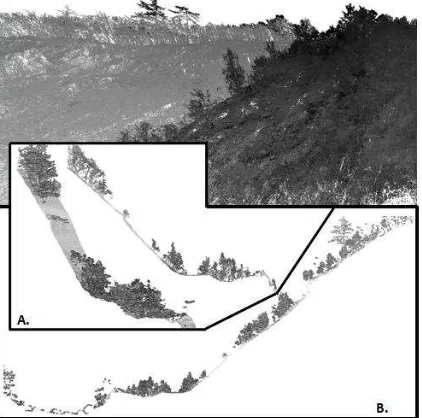
Figure 1. Multi-scale views of the study area.
There is an abundant presence of steppic vegetation, coppice, and high forest. This adds complexity to the scan as the vegetation does cover multiple strata above the ground ranging from low vegetation to high vegetation (Figure 2).
The the study area is located at 45°47'57.82" latitude and 11°20'15.01" longitude in the WGS-84 datum (area’s approximate barycentre). The overall slope and aspect in respect to the sensor position make for an advantage providing a high degree of visibility for the line of sight from sensor to objects.
Figure 2. 3D view of the acquired point data (top).
3. MATERIALS AND METHODS
3.1 Data acquisition
In this study we used a Riegl VZ-400 laser scanner, which uses time-of-flight range measurements with online waveform processing to record multiple return echoes. Table 1 shows the
instrument’s specifications.
Table 1. Specifications of the Riegl VZ-400. Field of view 100° x 360° Pulse rate up to 122000 Hz
Range up to 600 m
Repeatability 3 mm
Camera Possibility to be equipped with Nikon D700 or D300
Beam divergence 0.3 mrad
Spot size 3 cm at 100 m distance Minimum range 1.5 m
Laser wavelength Near infrared
The survey setup covered the entire area into seven scans with ranging from 10 to 75 million points each. For the presented work we chose the scan with the highest degree of area covered, with a total of 75.4 million points. Figure 3 shows a planimetric representation of the distance from the scanner of the recorded points with an overlap of the 5 transects used for checking the quality of the results (reported in section 3.3).
Figure 3. Range (meters) color scale of study site. Black lines represent transects used for quality control.
3.2 Data processing
Figure 4. Workflow of processing pipeline: PRN is point return number, NoR is total number of returns.
3.2.1 Terrain surface
The ground surface is important for successive vegetation assessment. Three variables are considered from the dataset to extract ground points: spatial coordinates, amplitude of the return signal and ordinal of return signal. The two last features are used in the first two steps to subset the total point cloud into candidate ground points.
The first step separates the points which belong to first or intermediate return echoes from the others, as they surely do not belong to the terrain (they actually can in a very limited number of cases which are considered not significant in the case of TLS because of its very narrow laser beam). All other points are considered candidate ground points. Amplitude is considered next. As mentioned in Axelsson (1999) it can be used as additional information on decision-making for this initial procedure. It can also be clearly seen on figure 2 (boxes A. and B.), as support to this approach, that the vegetation has a lower reflectance value respect to the terrain. This is more correctly said about leaves and small branches, as, upon closer inspection, the stem has a very similar amplitude value to the ground. Nevertheless the ability of filtering out leaves and branches still gives value to the amplitude information. The amplitude threshold to use (T) is determined by the first value of the last quartile of the cumulative distribution function of the amplitude values:
(1) The amplitude filter requires a threshold which has to be
calculated from the dataset’s amplitude frequency distribution
assuming that there is at least a minimal percentage of adapted here to the specific case of a TLS dataset. The dilation
and erosion operators (D and E) consider the maximum and minimum height (Z) values in a specific window of size C.
(2)
The window size is progressively decreased; the initial coarse resolution of the grid is 50 m. Nine successive passages doubles the resolution bringing the final grid resolution to ~0.1 m. The multi dimensional grids are pre-defined and all points are read through once, and are assessed in each grid-cell according to the operator. The process of merging the grids at the final resolution is applied after the cell values have been assigned from the points. The maximum admissible height difference which is accepted when progressively merging the grids as successive resolutions is based on the resolution itself and on the height of the nearest neighbours. This threshold is therefore progressive along with cell size; the new cell will not be assigned the new height if it is greater than the old resolution and if it is a local maximum respect to the eight neighbouring cells (both conditions must be true to discard the new height). This avoids “peaks” which are caused by commission errors in assigning a point as ground point when it belongs to vegetation.
3.2.2 Vegetation
A vegetation density index has been defined from Straatsma et al. (2008) with the difference of using all the space above each cell in the grid, and not spheric voxels. The vegetation density
where Nr is the total number of “hits” inside the space, Nt is the potential number of points that would be present if no before-hand occlusion was present and if the space reflected all incoming laser pulses and No are the number of points which got occluded by elements standing in between the sensor and the cell. This method does not account for pulses which do not cause any return because of very low target reflectivity or because they do not hit any target, but their number is negligible compared to the total number of points.
3.2.3 Delimitation of working area
The area to be considered for analysis in a TLS survey is not easily determinable because occlusions and distance from sensor cause heterogeneous point density. In this study the working area is determined in terms of the lowest acceptable point density found in each cell.
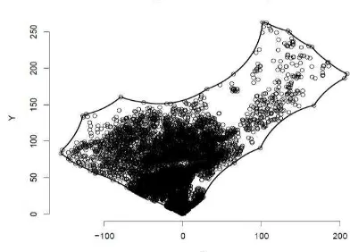
Figure 5. Working area from alpha cancave hull of points.
To define properly the model area we used a criteria based on alpha-hull definition (Pateiro and Rodr, 2010) to derive a concave-hull. Figure 5 shows results of applying the alpha-hull .
3.3 Accuracy assessment
The complex terrain and high vegetation density did not permit to conduct an efficient sampling on the ground to acquire ground truth measurements. For this reason the process of quality control for our method was carried out by extracting a DTM and DSM directly from the point cloud. Three transects (see figure 3) were taken by within a one-degree window on horizontal angle φ. This provided us with a strip with a 4.5 m width at its furthest point from the sensor (Figure 6 shows some extracted parts from the strips). The data to be used for control
was extracted partially with TerraSolid’s TerraScan, refined and controlled manually by visual interpretation, to extract a high resolution (0.1 m) DTM and DSM to be used as control. From these strips a DTM, a DSM and a set of 30 tree heights were extracted for calculating residuals. This was possible due to the high point density which allows visual interpretation and manual measurement as is clear in figure 6 which shows parts of the control transects.
Figure 6. Parts of the control transect used to check quality.
4. RESULTS AND DISCUSSION
The presented method gave consistent results. Figure 7 and 8 show the end-products, respectively the DTM, the vegetation density map and the canopy height model derived from the difference between the DSM and DTM.
Figure 7. The digital terrain model at 0.1 m resolution (meters).
Figure 8. A.) vegetation density mapping (n° of points belonging to vegetation/m2 B.) canopy height distribution (meters).
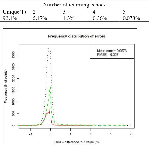
The consistency is shown in figure 9 where the distribution of the errors calculated by comparison between the data extracted from the transect samples and the estimation derived from our process. Not all three transects returned the same total area because the range of the data differed. The overall mean shows a small positive bias of around 5 cm, whereas the overall RMSE is about 30 cm. Table 2 below shows the mean and standard deviation of the differences for each transect.
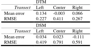
Table 2. DTM and DSM errors (m). DTM
Transect Left Center Right Mean error 0.134 -0.003 0.066
RMSE 0.227 0.411 0.267
DSM
Transect Left Center Right Mean error 0.034 0.023 -0.111
RMSE 0.419 0.791 0.591
The distributions of the errors for each transect have been tested against each other for proving the null hypothesis that they have been sampled from the same population. A t-test was used, and results indicated that the null hypothesis is not to be considered valid at a 95% confidence interval – thus suggesting an irregular distribution of the errors over the area. This result is quite reasonable considering the complexity of the terrain where in many parts we have a 90° slope. Therefore the overall mean and RMSE are to be considered only as indications.
Table 3. Percent of points per returning echoes
Number of returning echoes
Unique(1) 2 3 4 5
93.1% 5.17% 1.3% 0.36% 0.078%
Figure 9. Error frequency distribution of DTM. Continuous red, dashed green and dotted black lines respectively represent left, center and right transects.
Figure 10. Result of height differences over 30 trees.
Thirty trees have been measured directly from the point cloud to test the canopy height model (CHM) which was obtained from subtracting the DTM from the DSM. Sampled trees had a height between 5 and 12 m. Figure 10 reports absolute and relative errors – the former as the height difference for each tree and the latter as percentage of error referred to measured tree height represented using error bars. Overall mean of errors is close to zero and standard deviation of errors (RMSE) is 0.251 m. We see from the RMSE value that the expected error when extracting tree heights from the local maxima of the CHM would be more than 25 cm for about third of the measurements (if the error is normally distributed). Normality test (Shapiro-Wilk test at α = 0.05) confirms the normal distribution of errors with the exception of three outliers. The remaining 27 trees have an absolute error of less than 0.25 m, with a relative error ranging from 0.15%-7% of tree height. No significant correlation was found between relative error and corresponding tree height.
An important aspect of any procedure is the speed performance over very dense points. In terrestrial laser scanning this is a critical aspect, because datasets usually have a very high point density thus providing high detail but also potential redundancy when confronted with the end-product’s required level of detail. The consequence is that a high cost is paid over every additional step and iteration on the original point cloud. In this case the processing time can be estimated with the following parameters:
1
2i n
t O u
(4) where t is the total processing time for n points as a function of O which is the time it takes to stream through all the points and to process their three features used in the pipeline (Figure 4), u is the time taken to process the coarse first-level grid and i is the number of iterative increase in grid resolution (x2). In case that there is no information on the amplitude frequency distribution, this has to be calculated before-hand therefore streaming through all the points has to be done twice – the first for getting the information on the amplitude frequency distribution the second for the processing itself. The first iteration can take less time than the second if programming procedures are optimized.
5. CONCLUSIONS
Multi-return TLS sensors provide a higher point density and an increased ability to penetrate vegetation. These characteristics provide a higher number of samples when compared to single-return TLS. The very large amount of data requires investigation of processing methods which give accurate results without requiring extremely high computation time. This study reports on results of using a morphological filter to extract DTM and DSM layers and of a vegetation density estimation using the number of points belonging to vegetation accounting for occlusion. The difference between our method and the commonly used progressive triangulation method for DTM extraction is minimal (RMSE of around 30 cm with a mean of 0.0573 meters). Even if the difference is small, a further study of how this difference is distributed in space can be interesting to see if there is a correlation with point density, distance from sensor and/or the incidence angle between the laser diffraction cone and the object. An advantage which has to be further investigated is that it is less processing-intensive as it can use quadtree spatial indexing and can thus be optimized for speed,
random access memory limitation. Other methods are more calculation intensive; for example progressive triangulation requires spatially-oriented calculations to find if the candidate point satisfies the triangle’s minimum circum-circle criteria, and other steps to add the point to the mesh. The approach that we present here uses multi-resolutions regular grids thus allowing either a single pass over the whole point cloud or two in case there is no information on the amplitude distribution and the user wants to include that step in the procedure.
Derived CHM accuracy is compared with a manual measurement of tree heights and results show that the method gives most results with an absolute error below 20 cm, except for three outliers. Further investigation will be considered to understand the causes of high errors and eventual correlations with other characteristics such as range from sensor.
TLS sensor technology is improving in acquisition speed and data quantity/quality. This trend will likely continue, hopefully also decreasing costs. For these reasons research and testing of methods to extract information from TLS datasets is an important contribution to future development and implementation of practical tools.
REFERENCES
Axelsson, P., 1999. Processing of laser scanner data algorithms and applications. ISPRS Journal of Photogrammetry and Remote Sensing 54, 138–147.
Doneus, M., Pfennigbauer, M., Studnicka, N. and A. Ullrich, 2009. Terrestrial waveform laser scanning for documentation of cultural heritage. In: Proceeding of XXII CIPA Symposium, 11-15 October 2009, Kyoto (Japan).
Durrieu, S., Allouis, T., Fournier, R., Véga, C., Albrech, L 2008. Spatial quantification of vegetation density from terrestrial laser scanner data for characterization of 3D forest structure at plot level. In: Proceedings of SilviLaser 2008, Sept. 17-19, 2008 – Edinburgh, UK 325-334.
Guarnieri, A., Vettore A., Pirotti, F., Menenti, M., Marani, M. 2009. Retrieval of small-relief marsh morphology from Terrestrial Laser Scanner, optimal spatial filtering, and laser return intensity. Geomorphology, vol. 113; p. 12-20, ISSN: 0169-555X, doi: 10.1016/j.geomorph.2009.06.005
Haralick, R.M., Shapiro, L.G., 1992. Computer and Robot Vision. Addison-Wesley, Longman Publishing Co. Inc., Boston MA, USA.
Kraus, K., Pfeifer, N. 2001. Advanced DTM generation from LiDAR data. The International Archives of Photogrammetry and Remote Sensing 34(3/W4) , 23–30.
Lichti, D.D., Gordon, S.J. and Stewart, M.P., 2002. Ground-based laser scanners: operation, systems and applications. Geomatica, 56(1), 21-33.
Lichti, D.D. 2007. Error modelling, calibration and analysis of an AM–CW terrestrial laser scanner system. ISPRS Journal of Photogrammetry and Remote Sensing 61(5), 307–324.
Maas, H.G., Bienert, A., Scheller, S., Keane, E. 2008. Automatic forest inventory parameter determination from terrestrial laser scanner data. International Journal of Remote Sensing 29(5), 1579 – 1593.
Maas, H.G. 2010. Foresty Applications. Airborne and terrestrial laser scanning. Vosselman, G., Maas, H.G. Eds. First ed. Whittles Publishing, UK.
Mallet, C., Bretar, F. 2009. Full-waveform topographic lidar: State-of-the-art. ISPRS Journal of Photogrammetry and Remote Sensing, 64(1): 1-16.
Pateiro, B., Rodr, A. 2010. Generalizing the Convex Hull of a Sample: The R Package alphahull. Journal of Statistical Software, 35(5): 1-28.
Pfeifer, N., Winterhalder, D. 2004. Modelling of tree cross sections from terrestrial laser scanning data with free-form curves. The International Archives of Photogrammetry and Remote Sensing 36(8/W2), 76-81 .
Ramsay, J.O., Hooker, G., Graves, S. 2009. Functional Data Analysis with R and Matlab. Springer.
Sithole, G., Vosselman, G. 2004. Experimental comparison of filter algorithms for bare-earth extraction from airborne laser scanning point clouds. ISPRS Journal of Photogrammetry and Remote Sensing 59 (1-2), 85–101.
Stilla, U. 2011. Full Waveform Laserscanning Auswertung und ALS/TLS-Anwendungen. In: A. Grimm-Pitzinger, T. Weinold (ed.s), 16. Internationale Geodtische Woche Obergurgl 2011, Wichmann Verlag, Berlin (Germany), pp. 155-166.
Straatsma, M.W., Warmink, J.J., Middelkoop, H. 2008. Two novel methods for field measurements of hydrodynamic density of floodplain vegetation using terrestrial laser scanning and digital parallel photography. International Journal of Remote Sensing 29: 1595–1617.
Vosselman, G. 2000. Slope based filtering of laser altimetry data. The International Archives of Photogrammetry and Remote Sensing 33(B3), 935–942.