Handaru Jati, Ph.D
Universitas Negeri Yogyakarta
Chapter Overview
9.1 Introduction
9.2 Defining Simulation
9.2.1 Data Tables
9.2.2 Scenario Manager
9.2.3 Generating Random Numbers within Distributions
9.3 Applications
9.3.1 News Vendor Problem
9.3.2 Game of Craps
9.3.3 Bidding
9.4 Summary
9.1
Introduction
This chapter defines simulation and describes how simulation can be performed in Excel. We illustrate some simple tools available in Excel and then discuss how to use some new functions to create a simulation in Excel. The reader should be aware that there are several simulation software packages available that have more advanced features than what is available in Excel; since Excel is primarily a spreadsheet software, simulation features are not highlighted. However, we want to demonstrate, that when developing a spreadsheet-based DSS, simulation can be performed with the basic tools available in Excel. We revisit the simulation topic in Chapter 20 with VBA. We have several DSS applications which use simulation, such as Poker Simulation, Birthday Simulation, Queuing Simulation, and Reliability Analysis.
9.2
Defining Simulation
Simulation is a modeling tool that is used to imitate a real-world process and better understand system behavior. Authentic system behavior can be estimated through the use of distributions. From these distributions, a user can generate random numbers to evaluate multiple strategies and predict future performance. Simulation is a useful tool in that it can make observations through trial and error without the cost of materials, labor, and time that would be necessary to observe the same results of the original process.
For example, if the supervisor of a paper mill wants to determine how production will be affected by a change in the rate of raw material input, it would be very costly to observe the actual affects in the mill. He would have to instruct employees to change the rate of placing raw materials in the first machine, possibly change the processing times of some following machines, react to any malfunctions caused by this change, and possibly get an undesirable result, thus having to change everything back to how it originally was. By using simulation, he could see what would happen numerically without actually modifying the actual process. If the simulation model showed an increase in production by changing the rate of incoming raw materials, the supervisor could implement the change; otherwise, he would not need to waste time if production did not increase.
Simulation can be used differently from optimization in that instead of seeking to optimize an objective function value, it simulates the behavior of a system to assess its performance under several scenarios that may be used in “what-if” analysis. There are many applications in which simulation becomes useful; we will discuss these applications in the following sections. Excel offers two simple tools for performing simulation: Data Tables and the Scenario Manager. We will then explain how some Excel functions can be used to perform more advanced simulation.
9.2.1
Data Tablesoutput. For example, if you varied price and location values as input, you could observe profit. Since two inputs are changing, you would use a two-way data table.
To use Data Tables, you must first prepare your spreadsheet. To do this, create a list of inputs and outputs. These cells may contain values or formulas. You should label them for easy reference. Next, create a list of the various input values that you want to experiment with. If you are creating a one-way data table, you should put these values in a single column. If you are creating a two-way data table, you should create one column and one row of varying input values for the two inputs of interest. Then, enter the output formulas that you want the Data Table to calculate for observation. For one-way data tables, these output cells (again, more than one output can be observed using one-way data tables) should be in the columns adjacent to the input column. For two-way data tables, this output cell (again, only one output value is observed with two-way data tables) should be placed in the upper corner of the data table (in the cell above the column of input value and next to the row of input values).
Once you’ve prepared your spreadsheet, highlight the entire table area that you just created (without column or row titles). Now, select Data > Table from the Excel menu. A small dialog box will appear that asks you for the row and/or column input cell (see Figure 9.1).
Figure 9.1 The Row Input and Column Input cells refer to the initial list of inputs and outputs.
Let’s consider an example to illustrate both one-way and two-way data tables. In Figure 9.2, we provide a list of inputs and outputs for ticket sales. The Total Profit is calculated by finding the unit profit (price minus cost per ticket) and multiplying this value by the number of salespersons and the average number of tickets sold per person. Using the input cells shown, the formula for the total profit would be:
=(B6-B7)*B4*B5
Figure 9.2 The initial list of inputs and outputs contains values and formulas.
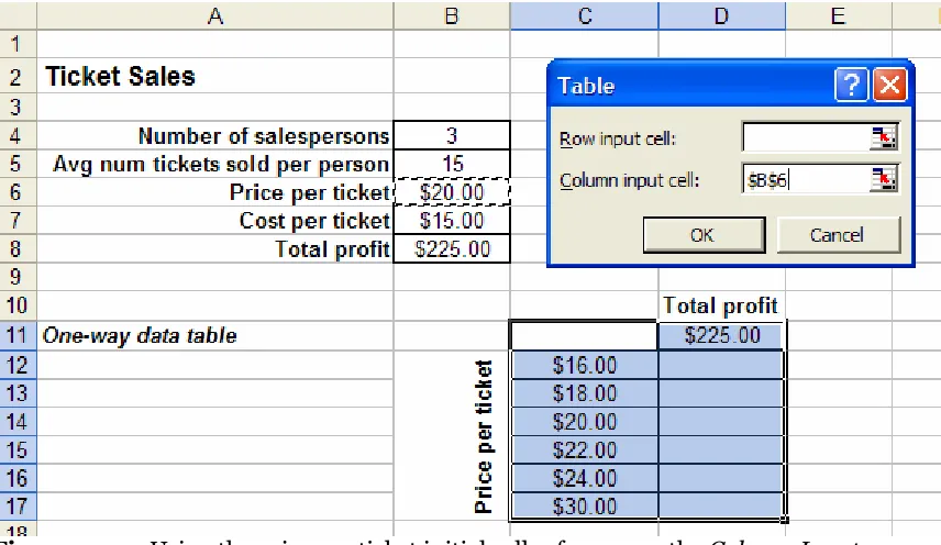
The first data table we want to create will show the different profit values as we vary the price per ticket. Since we are only varying one input, this will be a one-way data table. Let’s begin by creating a column of various prices per ticket. We will vary these prices from $16.00 to $24.00 per ticket. Then, we copy the formula used in cell B8 to a cell in the first row of the data table (above the first price value in the input columns). Note that the output formula can either be copied directly or we can just refer to the original formula cell in the list of inputs and outputs; that is, we could again type “=(B6-B7)*B4*B5” orsimply refer to this formula in the initial table by typing “=B8”. Figure 9.3 shows the preparation for this data table.
Figure 9.3 Preparation for the one-way data table comparing price per ticket and total profit.
Figure 9.4 Using the price per ticket initial cell reference as the Column Input.
Once we press OK, Excel completes the data table. In Figure 9.5, we find that various profit values have been calculated for each possible price per ticket listed.
Figure 9.5 The final data table shows various profit values as the price per ticket changes.
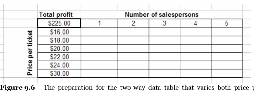
Figure 9.6 The preparation for the two-way data table that varies both price per ticket and number of salespersons.
We now select Data > Table from the menu. This time, we will reference both the Row Input and Column Input. The Row Input will be the number of salespersons, which is cell B4, in the initial list of inputs and outputs. The Column Input will again be cell B6 for price per ticket (see Figure 9.7).
Figure 9.7 The number of salespersons is the Row Input and the price per ticket is
the Column Input.
Figure 9.8 The final data table shows various profit values for combinations of number of salespersons and prices per ticket.
9.2.2
Scenario ManagerThe Scenario Manager allows you to vary up to 32 input cells for various values, or scenarios, and observe the results of several output cells. The Scenario Manager will create a Scenario Report, which shows the resulting output values for each scenario of input values.
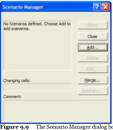
The spreadsheet preparation for using the Scenario Manager is simpler than that for Data Tables. All we need is the initial list of inputs or outputs. Appropriate values and formulas should be filled in in these cells. Now, we go to Tools > Scenarios to view the Scenario Manager dialog box shown below in Figure 9.9.
Figure 9.9 The Scenario Manager dialog box.
should be to the list of inputs created in the spreadsheet preparation. We also name the scenario at this time.
Figure 9.10 Creating the scenario name and selecting the input cells to change.
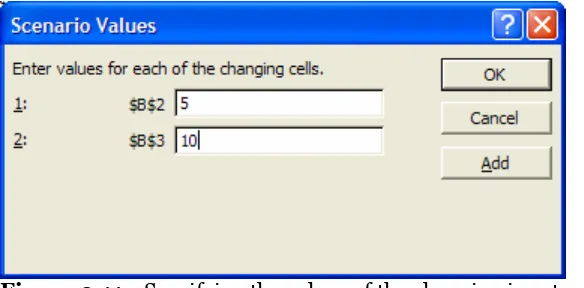
Next we specify the values that these inputs should take for the scenario that we are creating (see Figure 9.11).
Figure 9.11 Specifying the values of the changing input cells.
Figure 9.12 Selecting the output cells to put in the Scenario Report.
Let’s consider an example to illustrate the benefits of using the Scenario Manager. In the table shown in Figure 9.13, there is a list of inputs for a company’s sales. These inputs are: tax rate; Year 1 sales; sales growth; year 1 price; year 1 cost; interest rate; cost growth; and price growth. Then, there is a table of outputs for five years. The outputs are: unit sales; unit price; unit cost; revenue; costs; before tax profits; tax, after tax profits; and total NPV. The unit sales, unit price, and unit cost are actually inputs calculated using the growth rates from the input table.
Figure 9.13 The initial input and output cells.
Figure 9.14 Naming the Best Case scenario and selecting the changing input cells.
We select the input cells, or changing cells, for the year 1 sales, sales growth, and year 1 price: C5:C7. We name this scenario the Best Case scenario and give the values 20,000, 0.2, and 10 for these inputs, respectively (see Figure 9.15). Then, we press Add on this dialog box to directly create the next scenario.
Figure 9.15 Specifying the values for the Best Case inputs.
Let’s name this the Worst Case scenario and select the same input cells. We give them the values 5,000, 0.02, and 5, respectively.
Figure 9.16 Creating the three scenarios.
We now choose Summary and select the “after tax profit row” (for all five years), which is in cells C21 and G21, and the NPV cell, which is cell C23, as the outputs (see Figure 9.17). We then press OK to create the Scenario Report.
Figure 9.17 Selecting the output cells to create the Scenario Report.
Figure 9.18 The Scenario Report shows the outputs for the various input values in each scenario.
Note that we have named our input and output cells in order to see the names shown in the first column of the Scenario Report. If you do not name your cells, the cell reference will be shown instead (i.e. C23 instead of “NPV”). Also note that some icons are provided next to the row numbers and column letters to hide some parts of the report and to show others.
9.2.3
Generating Random Numbers within DistributionsDespite its benefits, creating many scenarios of possible input values with Data Tables or the Scenario Manager can be tedious. We will therefore explain how to use some important Excel functions to generate various input data values for several scenarios, or runs of a simulation.
Simulation is useful because it can handle variability of parameters in a model. That is, you may not know many settings in a process with full certainty; you may be aware of a range of numbers into which values fall, but not know the exact figures. For example, assume that there is a shipment company that is dependent upon a variety of suppliers before its workers can organize and ship their products. The company’s staff knows which suppliers will be delivering goods within a few days, but they do not know the exact day or time when each delivery will arrive. This variability affects their business, since they cannot satisfy their customers’ demands until they receive products from their suppliers. To put this situation into a model, we would not be able to assign a constant rate to the arrival of goods from suppliers. Therefore, we would want to study the arrival rates over a time and match the distribution to the arrival rate that closely matches the suppliers’ patterns. Once we know the distribution of a certain parameter, we can generate random numbers within this distribution to observe the effect on satisfying customer demand. Therefore, it is now appropriate to introduce the concepts of distributions and random numbers.
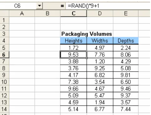
lower bound and n with the upper bound in the above formula. We demonstrate this particular use of RAND in in Figure 9.19 with n = 10. Here we want to generate heights, widths, and depths to calculate some probable packaging volumes. We type the following function to create random numbers between 1 and 10:
=RAND()*9 + 1
Figure 9.19 The RAND function can be manipulated to change the range of the random numbers produced. Here the range is changed from the default of 0 to 1, to 1 to
10.
We can convert these random numbers into random integers by changing the format of the cells in which we entered this function. Simply use the Number tab of the Formatting dialog box and set the number of decimal places to 0.
We can also generate a random integer by using the INT function with the RAND function. The INT function rounds a number down to the nearest integer.
=INT(number) =INT(range_name) =INT(cell_referenced)
=INT(RAND()*(n-1) + 1)
For example, the following formula would generate the numbers 1, 2, 3, 4 (random integers between 1 and 5):
=INT(RAND()*4 + 1)
Note that the integer 5 would never be generated using this formula since the INT function always rounds down to the nearest integer. That is, the random number 1.6 would be transformed to the integer 1. You could also use the TRUNC function to create an integer by removing the decimal part of a number without rounding. The TRUNC function is used similarly to the INT function.
An easier way to manipulate the RAND function is to use another function called RANDBETWEEN. This function takes two parameters, which are the lower and upper limits of the range. The format of this function is the following:
=RANDBETWEEN(lower_limit, upper_limit)
Note: to use the RANDBETWEEN function, you will need to ensure that the Analysis Toolpack has been selected as an Add-In. Go to Tools > Add-Ins to check.
Using the same example, if we wanted to create random numbers between 1 and 10, we would type the following:
=RANDBETWEEN(1,10)
Note: When using either RAND or RANDBETWEEN, the numbers generated will change with every operation performed in the worksheet. That is, after creating the table in Figure 9.19, if we were to then type new text or data into another cell on the same worksheet, the initial random numbers shown would automatically recalculate new random numbers in our range. To prevent this automatic recalculation from occurring, go to Tools > Options from the menu and, on the Calculation tab, check Manual. We can now use F9 to recalculate the random numbers if necessary. (Note, however, that some other functions may not recalculate automatically when copied after changing the Calculation option to Manual.)
The RAND and RANDBETWEEN functions can also be used with the distribution functions discussed in Chapter 7. The general distribution function has the following format:
=DIST(x_value, distribution_parameters, cumulative_value)
distribution, we would follow the next format:
=NORMINV(RAND(), mean, std dev)
In Figure 9.20, we have entered this function in a column of cells for a Normal distribution with a mean of 50 and a standard deviation of 15. The function is entered as the following:
=NORMINV(RAND(), 50, 15)
Note that most of the numbers generated are in the range between 35 (that is, 50 – 15) and 65 (that is, 50 + 15), with the majority being closer to 50.
9.3
Applications
We will now explain three common applications of simulation in Excel. To illustrate these examples, we will use the ideas of scenario analysis and random number generations in distributions. Please note that there are many other areas and models for which simulation is a beneficial tool besides the following.
9.3.1
News Vendor ProblemA bookstore must determine how many 2006 comic calendars to order in September of 2005. It costs $2.30 to order each calendar, and the store sells each one for $4.70. After January 1, 2006, any unsold calendars can be returned to the supplier for a salvage value of $0.75 each. Our best guess is that the number of calendars demanded is governed by the following probabilities:
So, how many calendars should the company order? Let’s set up our spreadsheet by listing the inputs and outputs. For inputs, you know the ordering cost, sales price, and salvage value. You are also provided with a table of possible demands with their corresponding probabilities (see Figure 9.21).
Demand Probability 150 0.3 200 0.3 250 0.4
Data Tables: Used to determine how outputs vary in response to changes in input.
Scenario Analysis: Performs all possible alternative actions and notes the varying results from these different situations.
Random Number Generation in Distributions: Use the RAND function as the first parameter in the inverse distribution functions.
Inverse Functions: NORMINV, LN or LOGINV (the Exponential inverse), BETAINV, BINOMINV, CHIINV, FINV, and GAMMAINV.
Figure 9.21 Preparing the spreadsheet using formulas to determine unknown values.
The expected number of magazines sold will be based on these demands and probabilities. First, we compute the cumulative probabilities of each demand (since demands are increasing). We then create a cell that will generate a random probability; we do this using the RAND function. To determine the expected number of magazines sold, we use the IF function to compare this random probability to the ranges of cumulative probabilities. We have named the cell ranges to make our formulas easier to read (see Figure 9.21).
We will then use the NORMINV function, combined with the RAND function, to determine how many calendars to order (see Figure 9.22). We set the mean to 200 (since this is the average demand) and the standard deviation to 15 (even though the standard deviation of the demand value is 50, we want to keep the order number closer to the mean).
Figure 9.22 Using the NORMINV function with the RAND function to generate a random number from the Normal distribution.
Figure 9.23 Making runs to compare profit values for several random input values.
This table displays 20 runs, or 20 rows of various input generated from changing random values. From the values stored in each run, we can easily find the average profit and average number of calendars ordered.
9.3.2
Game of CrapsIn the game of Craps, a player rolls two dice. If the first roll yields a sum of 2, 3, or 12, the player loses. If the first roll yields a sum of 7 or 11, the player wins. Otherwise, the player continues rolling the dice until she matches the value thrown on the first roll or rolls a sum of 7. Rolling a match for the first roll wins the game, rolling a value of 7 before a match loses the game. How many times will a player win on average in 1, 2, 3, 4, or 5 rolls?
Figure 9.24 The conditions for winning and losing on one or multiple rolls.
Let’s determine possible outcomes for 1, 2, 3, 4, and 5 rolls in a game. To do so, we will generate random results for rolling two dice for each roll for 20 games, or runs. To generate the result of a roll, we simply use the RANDBETWEEN function with the interval (2, 12). Then, we use the IF function to check the conditions for winning and losing and output the player’s status after the roll. For the first roll, we can use the following IF function (these cell references are for the first row in the simulation table):
=IF(OR(C26=2,C26=3,C26=12),"Lose",IF(OR(C26=7,C26=11),"Win", "Continue Play"))
Figure 9.25 Recording the outcome of rolling two dice for 20 different games.
For all sequential rolls, we again use the IF function, but this time, we are checking the current roll with the first roll. Therefore, we will need to create a new column for the second roll values (again using the RANDBETWEEN function) and compare these results with the results of the first roll value (see Figure 9.26). The comparative function with new winning and losing conditions can then be written as follows (these cell references are for the first row in the simulation table):
=IF(D26="Continue Play",IF(E26=$C26,"Win",IF(E26=7,"Lose", "Continue Play")),"")
Now, we can create two more columns (one for the roll value and one for the
Figure 9.26 Recording the number of wins when there are 1, 2, 3, 4, or 5 rolls in a game.
Now, we create a summary table below the simulation table. We want to count the number of wins for each roll among 20 games, or runs. To perform this conditional counting, we use the COUNTIF function. We will discuss this function in more detail in Chapter 10 with Database functions. The structure for this function is as follows:
=COUNTIF(table_range, condition)
For counting the number of wins in the first roll, we use this function:
=COUNTIF(D26:D45, “Win”)
We copy this formula to calculate the number of wins in each roll for all 20 games. What we have done is simply taken each of these resulting numbers and divided them by 20 to find the percentage of games won for each roll. (We can also press F9 to generate new rolls and simulate another 20 games, or runs, of data.)
9.3.3
BiddingNote that we could have also used the RANDBETWEEN function with this interval; however, we want non-integer values. Once we have generated possible bids for the competitors, we must determine possible bids for the contractor. She assumes that she will bid anywhere between $12,000 and $20,000 for the job. In this case, we have used the RANDBETWEEN function since it is just an estimate.
Now we can determine the output, which is the profit, by comparing the contractor’s bid to the competitors’ bids. If the contractor’s bid is the minimum value, then her profit is her bid minus her cost; however, if her bid is not the minimum, then she will lose the bid and not gain any profit (see Figure 9.27).
Figure 9.27 Calculating the inputs and output using several formulas.
Figure 9.28 Generating simulation runs to find the max profit.
When the 20 runs are complete, we can determine the max profit value by using the MAX function and the corresponding bid value. To find this bid value, we use the VLOOKUP function; however, since we are looking for the bid value based on the location of the max profit value, we must have the profit column in the first column of the lookup table. Therefore, we simply copy the bid column to the right of the profits and only select the data in columns F, G, and H as the lookup table. We can repeat this 20-run simulation by generating a new set of random numbers (by pressing F9) to compare the max profit and bid values.
9.4
Summary
¾ Simulation is a modeling tool used for analyzing a process running under different parameters.
¾ Simulation is used not to find the best result given certain inputs, but rather to find the best inputs given a desired result.
¾ Scenario Analysis performs all possible alternative actions and notes the varying results from these different situations.
¾ To perform random number generation in distributions, use the RAND() function as the first parameter in the inverse distribution functions.
¾ Inverse Distribution functions are the following: NORMINV, LN (the Exponential inverse), BETAINV, BINOMINV.
6. Name four of the inverse distribution functions under the Statistical category of functions in Excel.
7. How can you generate a random number within a distribution?
8. Which inverse distribution function is appropriate to use for generating a random number within an Exponential distribution?
9. If given a gamma distribution with an alpha value of 5 and a beta value of 8, what is the appropriate functional expression to generate a random number?
10. Give an example of an application of Excel simulation.
9.5.2
Hands-On Exercises1. A student needs a grade average of at least 93.0 points to receive an A in one of his classes. The student’s grade average is computed by averaging the
student’s score on five different tests given in the class. Each test is scored out of 100 points, and the highest grade the student can receive is 100 points since no extra credit is offered. The student received the following grades on the first three tests: 86, 94, and 88. He is trying to determine if it is possible for him to earn an A in the class and if so, what grades he must earn on the final two tests in order to earn an A. Perform an Excel scenario analysis to determine if the student can possibly receive an A in the class, and, if he can, determine what combinations of grades on the final two tests will enable him to do so.
2. Generate five random numbers for each of the following distributions:
a. Exponential distribution with a mean of 12 and a standard deviation of 2. b. Beta distribution with an alpha of 4 and a beta of 3.
c. Chi-squared distribution with 6 degrees of freedom. d. Standard normal cumulative distribution.
3. In chapter 4, problem 3, you completed the following table, which determines the height of a cylinder given its volume and radius. Use scenario analysis to
4. A bakery receives its ingredients from one of three vendors. Each vendor under consideration charges different prices for each different ingredient. The tax rates vary by the state in which the vendors are located, and the shipping costs vary by the distances the supply must travel. The table below displays the prices, tax rates, and shipping costs per pound for each vendor. The management has to choose a vendor for each ingredient. It has been estimated that 200 lbs of ingredients will be needed per month. Use scenario analysis to help the management to choose a vendor for each ingredient.
Vendor A Vendor B Vendor C
5. A materials engineer is conducting a test on the fracture toughness of an expensive ceramic material. The engineer wants to report on the results of fifty trials but can only afford to actually conduct ten trials since testing the material renders it unusable. Her results so far have followed a chi-squared distribution with 3.5 degrees of freedom. Using random number generation, predict forty more possible trial results for the engineer to use.
6. A company is opening up a new distribution center in Gainesville, Florida. Five different banks have offered the company loan plans; each plan’s cash flow is provided below. Initially assume that the interest rate is 5%.
a. Create a spreadsheet that finds the net present value and the internal rate of return of each loan.
b. Run several scenarios that change the interest rate to 3%, 3.5%, 4%, and 4.5%. c. View the scenario summary. Which interest rate would the company prefer?
Which bank can provide the most economical loan plan for the company?
Year Bank A Bank B Bank C Bank D Bank E
0 $1,000,000 $1,000,000 $1,000,000 $1,000,000 $1,000,000
1 -$100,000 0 -$150,000 0 -$500,000
2 -$200,000 -$300,000 -$150,000 0 -$100,000 3 -$300,000 -$300,000 -$150,000 0 -$100,000 4 -$400,000 -$300,000 -$150,000 0 -$100,000 5 -$500,000 -$300,000 -$150,000 -$250,000 -$100,000 6 0 -$300,000 -$150,000 -$250,000 -$100,000
7 0 0 -$150,000 -$250,000 -$100,000
8 0 0 -$150,000 -$250,000 0
9 0 0 -$150,000 -$250,000 0
boxes should be processed before the blades on the Flex-O machine should be replaced? Use ten scenarios with thirty runs each and find the minimum value to approximate the number of boxes to produce before replacing the blade. Your objective is to use each blade as long as possible but change it before failures start to occur.
8. A PVC pipe manufacturer has recently approximated the effect of certain factors on the amount of time it takes to produce a certain length of PVC pipe. These factors include the pressure and temperature of the liquid PVC and the radius and thickness of the pipe. The time that it takes to produce PVC pipe is shortest when the liquid PVC pressure is at 20 psi, the liquid PVC temperature is 240 degrees Fahrenheit, the radius is at its minimum setting of one-half inch, and the thickness of the pipe is at its minimum setting of one-eighth inch. The time to produce a 12-foot pipe at these settings follows a normal distribution with a mean of 85 seconds and a standard deviation of six seconds. Below are the
approximated effects of each factor on the mean time necessary to produce a 12-foot PVC pipe. Note that P is the liquid PVC pressure setting, T is the liquid PVC temperature setting, R is the radius of the pipe, and TH is the thickness of the pipe.
Liquid PVC pressure factor = 1 + (20 – P)/(20 * 10) Liquid PVC temperature factor = 1 + (240 – T)/(240 * 10) Radius factor = 1 + (R – 0.5)/(0.5 * 10)
Thickness factor = 1 + (TH – 0.125)/(0.125 * 10)
Use scenario analysis to find the approximate time to produce a 12-foot PVC pipe for each of the following settings:
a. P = 21 psi, T = 230° F, R = 1”, TH = 0.25 b. P = 18 psi, T = 250° F, R = 2”, TH = 0.35 c. P = 24 psi, T = 235° F, R = 5”, TH = 0.5 d. P = 17 psi, T = 245° F, R = 3”, TH = 0.25
manager would like to order all of the products at an appropriate time so that they will arrive in time to meet demand without accumulating too much. After studying past trends, the distribution manager approximated the distributions of the
demand rate and supply time for one of the products as shown in the following table. Assume that the product is perishable and only good for the month in which it is ordered. Also assume that the product is ordered in batches of 100. The supply time follows a normal distribution with the following parameters:
Mean = ceiling[20 * (1 + (D – 200) / 200)], where D is the amount of demand
a. Use ten runs to find the approximate number of batches to order to meet the demand and the approximate number of days to allow for delivery so that the delivery will arrive in time for the next month.
b. Perform scenario analysis to find the results for each of the following distributions if the time of supply arrival has a Normal distribution with the following parameters:
10. A local company currently sells 40,000 units of a product for $45 each. The unit variable cost of production for the product is $5. The company is thinking about cutting the product price by 30%. They are sure this will increase sales by an amount between 10% and 50%. Perform a sensitivity analysis to show how profit will change as a function of the percentage increase in sales (ignore fixed costs):
a. Using Data Tables
wins. What is the probability that the player will win?
13. Suppose you are bidding for an oil well that you believe will yield $40 million (including the cost of developing and mining the oil) in profits. Three competitors are bidding against you and each competitor’s bid is assumed to follow a normal random variable with a mean of $30 million and a standard deviation of $4 million. What should you bid (within $1 million)?
14. Two basketball teams are ready for the best-of-seven NBA finals. The two teams are evenly matched, but the home team wins 60% of the games between the two teams. The sequence of home and away games is to be chosen by Team A. Team A has the home edge and will be the home team for four of the seven games. They have the following sequence choices for the home games:
a. Sequence 1: Team A, A, B, B, A, B, A b. Sequence 2: Team A, A, B, B, B, A, A
Use simulation to prove that each sequence gives Team A the same chance of winning.
15. The game of Chuck-a-Luck is played as follows: You pick a number between 1 and 6 and toss three dice. If your number does not appear on any of the dice, you lose $1. If your number appears x times you win $x. On the average, how much money will you win or lose on each play of the game?
16. In August 2004, a car dealer is trying to determine how many 2005 cars should be ordered. Each car ordered in August 2004 costs $10,000. The demand for the dealer’s 2005 models has the probability distribution shown in the table below:
Cars Demanded Probability
20 .30 25 .20 30 .25 40 .25
determine how many cars should be ordered in August 2004. For your optimal order quantity, find the expected profit.
17. In the above problem, suppose now that the demand for cars is normally distributed with a mean of 40 and a standard deviation of 7. Use simulation to determine an optimal order quantity. For this optimal order quantity, determine the expected profit.
18. A ticket from Miami to Orlando sells for $150. The plain can hold 100 people. It costs $8,000 to fly an empty plain. The airline incurs variable costs of $30 per person on the plane. If the flight is overbooked, anyone who cannot get a seat receives $300 in compensation. On the average, 95% of all people who have a reservation show up for the flight. To maximize the expected profit, how many reservations for the flight should be taken?
19. An emergency room at a nearby hospital has an average of 2 patients arriving every hour (exponentially distributed). Upon entering, each patient fills out a form; this always takes 5 minutes. Then, each patient is processed by one of two registration clerks. This takes an average of 7 minutes (exponentially distributed). Then each patient walks 2 minutes to a waiting room and waits to meet the doctor. The time it takes the doctor to see a patient averages 20 minutes with a standard deviation of 10 minutes (normally distributed).
a. On average, how long does a patient spend in the emergency room? b. On average, how much of this time is spent waiting for a doctor? c. What percentage of the time is the doctor busy?
20. A person plays a game in which 2 fair dices are thrown. If the total outcome is 7 or 11, the person wins the game. Use simulation to find the probability of a win.
21. Jane is buying a house that costs $210,000. A financial institution is willing to lend her the money. The bank provides different rates depending on the amount of down payment and the duration of the loan. The table below presents the interest rate for different loan durations and amount of down payment. Use two-way Data Tables to calculate the monthly payments that Jane will be making to pay-off the loan under each scenario.
Loan Duration (in years)
The manager of the restaurant would like to perform a simulation analysis to see if hiring new employees would be beneficial.
a. Simulate the arrival and service time of 100 customers using the information provided above.
b. Estimate the expected waiting time per customer, expected total time in the system, the longest waiting time, and the percentage of time the server (drive through window) is idle.
c. Assume that one additional employee was hired. Recalculate the expected waiting time per customer, expected total time in the system, the longest waiting time, and the percentage of time the server is idle.
23. The coffee shop in a university town faces the problem of many bagels to order per day from a nearby bakery. For planning purposes, the bakery requires that a fixed amount of bagels be ordered every day in a given month. At the end of the month, the order size may be changed.
Based on past observations, the coffee shop manager has identified the following distribution of daily demand for bagels for the current month:
It costs $0.1 to buy a bagel from the bakery, regardless of the quantity ordered. The bagels are sold for $1.05. Left over bagels are disposed at the end of the day. The manager is interested to identify an order size for the current month that would maximize the profits.
Randomly generate the demand for the 30 days of the current month using the distribution given above. Consider order sizes from 20 to 40. For each order size,
calculates the corresponding profits. Based on the results of the simulation what should the order size for the current month be?
24. The tables below present the distribution of the inter-arrival time and service time of the jobs in a service center.
Time between arrivals Probability 30 minutes 0.20
45 0.35 60 0.25 75 0.15 90 0.05 Total 1
Estimate the expected waiting time per job, expected total time in the service center, and the longest waiting time for 100 jobs under the following two different service rules:
First In First Out (FIFO) – jobs are served in the order they arrive. Last In First Out (LIFO) – the last job to arrive
Service time Probability 20
minutes
0.15