Handaru Jati, Ph.D
Universitas Negeri Yogyakarta
Chapter Overview
10.1 Introduction
10.2 Importing Data
10.2.1 Text Files
10.2.2 Web Addresses
10.2.3 Databases
10.3 Exporting Data
10.4 Creating Pivot Tables from External Data
10.5 Using Excel as a Database
10.5.1 Sorting
10.5.2 Filtering
10.5.3 DFunctions
10.5.4 Data Validation
10.5.5 Data Consolidation
10.6 Summary
10.7 Exercises
10.1
Introduction
This chapter explains how to work with external data or large data in Excel. We illustrate how to import data from text files, webpages, and databases. For the database discussion, we assume the reader has some previous knowledge about database software, such as Microsoft Access. Knowing how to import data to the spreadsheet environment is an important attribute for developing a DSS. In many real-life applications, large amounts of data will be stored in a separate database; this data has to be imported as input for the model in the DSS. We revisit this topic in Chapter 21 to illustrate how this can be done using VBA. We have developed several DSS applications which use these features, such as the University Information System application.
10.2
Importing Data
Excel offers many tools for working with and analyzing large amounts of data. In many cases, an Excel user may not be given data in a worksheet to manipulate. If this is the case, you can use the Import options in Excel to transfer this data to a worksheet where Excel analysis tools can be applied. There are three sources from which you can import data into Excel: a text file, a webpage, and a database.
10.2.1 Text Files
To import data from a text file, use the Text Import Wizard. If you try to open a text file in Excel, this Wizard will appear. There are three simple steps to follow to use the Wizard. The first step is to specify how you want to organize your data into columns for Excel. There are two main options: Fixed Width and Delimited. If you choose Fixed Width, Excel will guess how to separate your data into columns. The second step of the Wizard will then give you a chance to modify this guess. If you choose the Delimited option, you specify what character will be used as a separator, for example: commas, spaces, tabs, etc. This character choice would be done in the second step of the Wizard with the
Delimited option. The third step of the Wizard in both cases is to specify any particular numerical formatting to be applied to the data as it is imported into Excel. Let’s take a closer look at the Text Import Wizard through an example:
Figure 10.1 Text file of employee hours.
The supervisor of these employees may be interested in calculating the average hours worked per employee and the average hours worked every Monday. To take advantage of Excel tools and functions that will help her accomplish this, she must import this text file into Excel. After ensuring the above data is saved as a text file, we open Excel and choose File > Open from the menu; then select the above text file. The Text Import Wizard will appear (see Figure 10.2).
Figure 10.2 Step 1 of the Text Import Wizard.
Figure 10.3 Step 2 of the Text Import Wizard.
Figure 10.4 Step 3 of the Text Import Wizard.
We are now done with the Text Import Wizard; the text data should now be imported into Excel columns, as shown in Figure 10.5.
Figure 10.5 The text file data imported into Excel columns.
Figure 10.6 The final organized data with average calculations.
10.2.2
Web Addresses
To import data from a webpage, use the Data > Import External Data > New Web Query
option from the menu. In the dialog box that appears, you can enter the web address that contains the data you want to import. There will then be a preview of this website in the window. You can then select what sections of data you want to import; that is, you may not want to import everything on the webpage. The possible data sections will be marked by small arrows. Select the arrows for all the data you are interested in and then click Import. Excel will prompt you to select a cell in the worksheet for where you want to place this imported data. Excel will import the data and separate it into columns, as done on the webpage. There is no prompt for how to separate this data, but Excel usually makes a good guess. You can always reorganize your data in the spreadsheet, if desired.
Let’s consider an example. The following web address contains current stock quotes and information for MSFT stock (see Figure 10.7), reported by Quicken:
Figure 10.7 Quicken quote on MSFT stock.
Figure 10.8 Web query for the MSFT quote information.
In the above webpage preview, we can see the small arrows in yellow boxes that Excel has placed on different sections of data. Since we are only interested in the actual stock data, we select the arrow next to “Last Trade.” Notice as you place your cursor on this arrow that a square appears around the entire section of data associated with that arrow. After we click the arrow, it will become a check mark, indicating that we wish to import this data. Now that we are done selecting data, we click Import. Finally, we must specify where in the worksheet we would like to paste the data (see Figure 10.9).
The data has now been transferred to the worksheet, as seen in Figure 10.10. Excel has also formed appropriate columns.
Figure 10.10 Imported data is separated into columns.
We can now further format this data for future analysis. We have added a title to the table and left a place to enter the date and time when this query was made (see Figure 10.11). We may then keep a record of “Last Trade” values, or others, as we continue to repeat this query in the future. To repeat a query, use the Refresh Data option from the
Data menu. Simply select the range of queried data in the worksheet and select Data > Refresh Data from the menu. Any changes on the webpage will be reflected on your worksheet.
Figure 10.11 The web data is organized for analysis.
10.2.3
Databases
To import data from a database, choose Data > Import External Data from the menu. From here you can browse to find a database file with which you want to work. These files do not need to be other Excel files; they can be any Data Access Object or ActiveX Data Object. The options available to you at this point will all involve an understanding of databases.
Excel, we prepare a new worksheet. First, we choose Data > Import External Data from the menu; the window in Figure 10.12 will appear.
Figure 10.12 To import data, choose Data > Import External Data from the menu and specify where to place the data.
We then specify where we want the imported data to be located. In this case, we choose a cell in the worksheet, say B4, and press OK. The imported data will then be copied to the worksheet, as illustrated in Figure 10.13. Notice that an External Data toolbar automatically appears next to the data. The first two options on the toolbar are
Edit Query and Data Range Properties. Edit Query allows us to modify what part of the database we have imported. A query is a search for a particular set of data from the database; it is similar to filtering. The Data Range Properties option gives us the opportunity to fine-tune the data before us. We can also update the data by using the
icon. The icon will ensure that any changes that have been made to the original database are reflected in our Excel worksheet.
Figure 10.13 The data has now been imported into the worksheet in Excel.
Figure 10.14 To choose a data source, we need to specify the type of database we are using.
The next window will provide a list of files that match this data source type (see Figure 10.15). In the list, we should find the file, books.mdb; we select it and press OK. Now, we begin to define our query.
Figure 10.16 Selecting which columns of data we want to appear in our final table.
Now, we specify how we want to filter this data. This is the query definition (see Figure 10.17). First, we select the column title, or field, by which we want to filter our data. Then, we select an equality type and a value from that field. In this case, we decide to filter the data by selecting all entries whose Copyright Year is equal to 2000 and click
Next. Note that we can have multiple filters among each available field.
Figure 10.17 Filtering data is how to define a query. We can select one or more fields, equality and a value from the field(s) by which we want to filter the data.
Figure 10.18 Specifying how to sort the data in the final table.
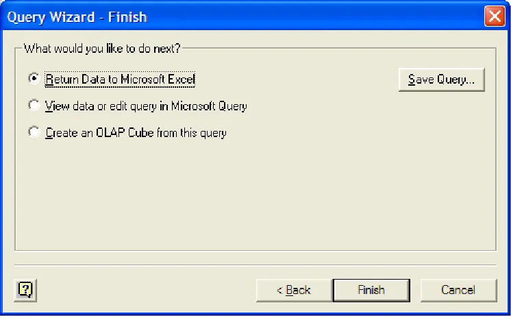
After pressing Next, we arrive at the last step in creating our query. This step requires us to decide whether we want to place the data from this query in Excel, view it in its original data source, or create an OLAP cube. The first two options are the most commonly used; we will view our data in Excel (see Figure 10.19). To view the final table, we click Finish.
Figure 10.19 Selecting to view the results of the query in Excel.
needed (refer to Figure 10.20). Notice here that only the books with Copyright Year of
2000 are shown in the table and that all of the books are sorted alphabetically by Author.
Figure 10.20 Formatting data in a table to use in our worksheet.
Databases constitute an important part of Excel applications. Involving VBA code in database applications extends your options in organizing your data.
10.3
Exporting Data
After working with a database in an Excel worksheet, you can export data to another workbook or to a database in another program. To export data from Excel to a database, you have to use an Add-In called AccessLinks. This Add-In must be downloaded and installed from the Microsoft webpage: http://www.microsoft.com/downloads. (The only valid database available to export using this Add-In is Microsoft Access.) Once it is installed, simply go to the Data menu option and select from the three exporting methods: MS Access Form, MS Access Report, or Convert to MS Access (see Figure 10.21).
10.4
Creating Pivot Tables from External Data
When we discussed Pivot Tables in Chapter 6, we mentioned that you can use data not only in your spreadsheet, but also from an external data source. In the first step of the Pivot Table Wizard, we select the type of data that we want to use (see Figure 10.22). To use external data, select External data source from the list of options.
Figure 10.22 Choosing external data as the source of the pivot table.
We will then be prompted to select the actual data (see Figure 10.23). To specify the data type and location, we click Get Data.
Figure 10.23 Getting the actual data to use for the pivot table.
Figure 10.24 Selecting the MS Access Database data type.
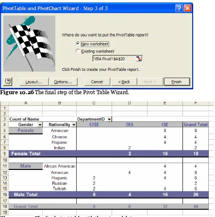
We are now prompted to choose the data within our data source to use for the pivot table (see Figure 10.25). In this example database, we have several tables and queries of data for a University System Database. Let’s look at the data in the Student Table to make an analysis of the number of students of each nationality and gender by using a pivot table. We select the Student Table from the left window and click the + icon. Then, we select the field names, or column titles, that we are interested in and click the > arrow to move them to the right window. All of the fields listed in the right window will be imported to the pivot table.
Figure 10.25 Selecting the table fields to be imported to the pivot table.
Figure 10.26 The final step of the Pivot Table Wizard.
Figure 10.27 The final pivot table with the external data.
10.5
Using Excel as a Database
Excel defines any well-defined table of items grouped by similar categories as a
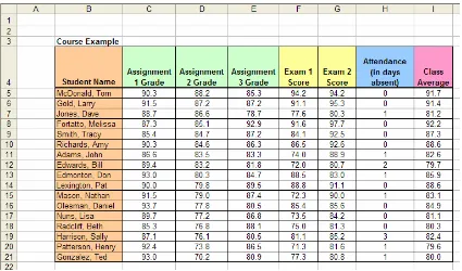
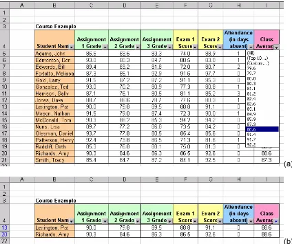
database. For example, a teaching assistant for a course may develop a detailed table of student records; he could consider this table a database. In this database, he can store the students’ names, homework grades, exam scores, and attendance, and he can also calculate their class average in the same table (see Figure 10.28). The basic menu options provide several simple functions that can be performed on Excel databases.
The first database function we will discuss is sorting. To sort means to order all entries in a database by a particular field; a field is a category name. (In Figure 10.28, each column heading of the table is a database field name.) In the example shown in Figure 10.28, we see that the names of the students are in no particular order. To place the names in alphabetical order, We can sort the entire database by the field of Student Name.
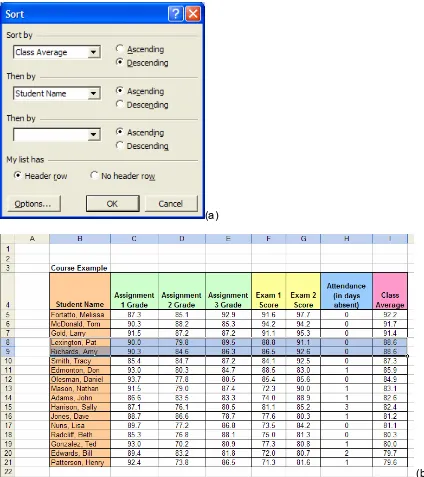
Figure 10.28 This database of student records for a course contains eight fields.
To do so, we highlight the entire database, including the field names; this is the range
B4:I21. Next,we choose Data > Sort from the menu. We will then see a window similar to Figure 10.29.
Figure 10.29 (a) The Sort window allows us to choose a field name by which to sort and select Ascending or Descending Order for the sort. (b) A list of all of the field names.
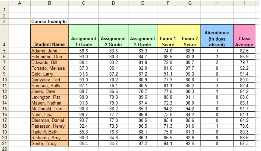
We can select any field name to sort by; we have chosen Student Name in Ascending Order. Ascending Order will list last names from A to Z; Descending Order would list them in the opposite order. We can see the results of this sort in Figure 10.30. Note
that the and icons at the top of the window will automatically sort the highlighted database by the first field in Ascending and DescendingOrder, respectively.
(a)
(b) Figure 10.31 First sorting by Class Average in Descending Order and then by Student Name in AscendingOrder. (b) The database is now sorted.
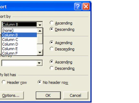
Figure 10.32 If we select No header row, the Excel column names are used as field names instead of as column titles in the database.
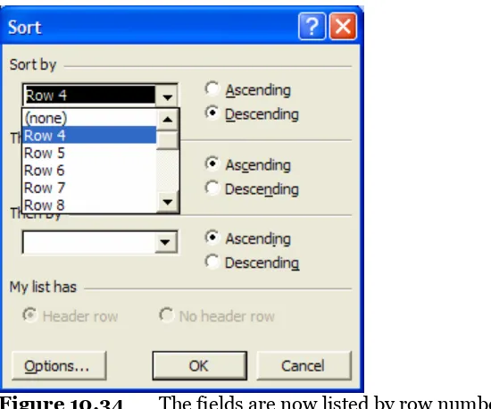
We can also sort within a row. To do this, we click the Options button on the Sort window. The window shown in Figure 10.33 appears. There is an option to determine how the first field we sort by should be sorted; the default value is Normal; other options refer to date values. We can also select whether our data is Case Sensitive or not. To sort within a row, we will need to change the Orientation option from “top to bottom” to “left to right.”
Figure 10.33 Sort Options include sorting from top to bottom or left to right.
Figure 10.34 The fields are now listed by row number.
Using the student data, let’s choose row 4 to sort by since it has the titles of the different grades. If we sort by Row 4 in Ascending order, we will see the table shown in Figure 10.35.
Figure 10.35 The table is now sorted by row 4.
Sorting is a useful database function as it allows us to organize our data in multiple ways. It becomes even more valuable as the size of our database grows. It can also function as a search tool. For example, it can help us find an item name in an alphabetical listing.
10.5.2 Filtering
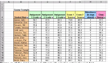
The next database function we will discuss is filtering. Filtering differs from sorting in that it selects a specified set of data from the database instead of ordering the entire database. Filtering allows you to select a group of entries in a database that is equal to a particular data entry within a field. For example, referring to Figure 10.28, instead of ordering all of the data by sorting by Class Average, we could select to view only the row items that have a Class Average equal to 88.6. To do so, we begin by highlighting the entire database, including column titles, cells B4:I21. Then,we choose Data > Filter > Auto Filter from the menu. This selection will transform the database by adding drop-down arrows to each field (see Figure 10.36).
Figure 10.36 The database is auto-filtered with selection options for each field.
We then select the arrow attached to the Class Average field. Here, we determine a particular data value, say 88.6, that will reconstruct the database so that it only displays the rows whose Class Average entries match the value chosen (see Figure 10.37). We can again display the entire database by clicking on the option arrow of Class Average
(a)
(b) Figure 10.37 (a) Selecting the drop-down list of values in the Class Average field. (b)The database is filtered to only show data entries with a Class Average equal to 88.6. There are two more options on the filtered drop-down list in each field that we would like to discuss. One is Top 10 and the other is Custom. Selecting Top 10 allows us to display 10 entries (or another specified amount) or 10 percent (or another specified percent) of the entries on the top or bottom of the database. In Figure 10.38, we chose to show the top 10 entries.
(b) Figure 10.38 Choosing the Top 10 option from the drop-down list. (a) Specifying
Top or Bottom, a certain number, and items or percent. (b) The database is updated to show only the number of entries specified.
The Custom option gives you a set of inequality specifications. You can choose to view entries whose field value is less than, greater than, or equal to a certain value. There is also an And/Or option which allows you to narrow your search to a particular range of values. For example, in Figure 10.39, we have specified to list only the entries whose
Class Average is between the values 81.1 and 82.4.
(a)
(b) Figure 10.39 Selecting the Custom option. (a) Specifying to show only entries with
Filtering is useful for locating specific data correlations in a database. You can define a select group of data by choosing a field entry that they have in common. There are many applications of databases for which filtering will be a necessary tool.
10.5.3 DFunctions
There is a group of Excel functions that are meant specifically for working with Excel as a database; we call these functions Dfunctions. These are specific functions designed for use with databases. They include DSUM, DAVERAGE, DMIN, and DMAX, which are essentially the same functions as SUM, AVERAGE, MIN and MAX, which we discussed in Chapter 4. Dfunctions differ from the previously described functions because they specify certain criteria before performing the function. That is, the formats of these functions have extra parameters (we use DSUM to illustrate the general format):
=DSUM(database, field, criteria)
The criteria parameter must include a field name and a criteria cell. In preparation for using Dfunctions, we must add a few rows to our database (see Figure 10.40). These rows contain our criteria and must repeat our field names. We will define the Dfunction
for this example in a new cell below these criteria. Using the example from Figure 10.28 one more time, let’s find the minimum Exam 2 score for students with a Class Average
above 85.0.
To do this, we choose Insert > Function from the menu, or select the fx icon from the standard toolbar and find the function category labeled Database. We can now view all of the Dfunctions and choose DMIN from the list (see Figure 10.41). After selecting DMIN, a new window will appear that guides us through defining the function.
Figure 10.41 In the function window, selecting the Database category to view all
Dfunctions.
Here we begin by defining the database parameter, which is the entire database excluding the new criteria rows, cells B3:I20. The field parameter is the name of the field in which we are searching for a minimum value, in this case, the Exam 2 Score. We specify the minimum value by entering the cell with this field name, which is G3. (We could also just enter the title of the field here.) Lastly, the criteria parameter includes the field name and criteria value cells. In this scenario, we want to find the minimum Exam 2
score for only the students with a Class Average above 85. Therefore, in the criteria cells, >85 is the criterion in the Class Average field. So for this parameter, we enter the cells I21:I22. The final DMIN function is then as follows (also see Figure 10.42):
Figure 10.42 Each argument is defined here for the DMIN function. Explanations of each argument are provided below the entry fields.
After entering this Dfunction, we will find the minimum Exam 2 Score to be 91 (see Figure 10.43(a)).
We have illustrated another scenario that searches for the minimum Exam 2 Score for the students with exactly 1 absence. In this case, the number 1 is the criterion for the
Attendance field. Notice that the DMIN function in this case has the same database and
field parameters but different criteria since we are now reviewing a condition in the
Attendance field instead of the Class Average field (see Figure 10.43(b)).
(a)
(b)
The other Dfunctions can be defined in a similar fashion. After clicking the fx icon and choosing a Dfunction from the Database category, the Function Argument window will guide you through defining your database and criteria for which you want to perform the selected function. Dfunctions are useful for databases as they allow you to consider many options in your search for a particular value.
Some other functions that are not Dfunctions are also useful to manage database data in Excel. One group of these functions, COUNT functions, has four main sub-functions: COUNT, COUNTA, COUNTBLANK, and COUNTIF. The COUNT function simply counts the number of cells with numerical values in a given range. The format of the function is as follows:
=COUNT(range)
The COUNTA function counts all of the cells with data of any kind in a given range of cells. That is, it will count the number of cells with numbers or text, or any other non-blank cell. The format for this function is:
=COUNTA(range)
The COUNTBLANK function counts the number of blank cells in a given range. It can be helpful for finding empty entries in a data table. The format for this function is:
=COUNTBLANK(range)
Let’s use these three functions on the student data in the previous example. Suppose we want to determine the number of assignments in the record. To use the COUNT function, we must highlight a row of grades, excluding the row of assignment titles. We must exclude the row of assignment titles because the COUNT function only counts cells with numerical values. If we use the COUNT function with the cells C4:G4, we find that 5 assignments have been recorded. To count the number of students in the class, we can use the COUNTA function with the first column of data (B4:B20); the result is 17 students.
Now suppose that we want to determine the number of students who never had an absence. We can remove the “0”s from the column of absences so that there are blanks instead. Now we can use the COUNTBLANK function with the attendance column (H4:H20); the result is that 9 students have perfect attendance records. See Figure 10.44 for these results.
Dfunctions: Functions with extra criteria specified for database use.
DSUM, DAVERAGE, DMIN, DMAX
Figure 10.44 Using the COUNT, COUNTA, and COUNTBLANK functions.
The COUNTIF function is probably the most useful COUNT function. It counts the number of cells in a given range that meet a specified criterion. The format for this function is:
=COUNTIF(range, criterion)
The criterion can contain some helpful characters such as * for a sequence of unknown values or ? as a single wild card value.
Let’s use the COUNTIF function to determine the number of students who have an A (≥ 90), a B+ (≥ 85), or a B (≥ 80) as their final grades. First, we need to find the number of students with an A by using the COUNTIF function as follows:
=COUNTIF(I4:I20, “>=90”)
Figure 10.45 Using The COUNTIF function with the student data.
Similar to the COUNTIF function is the SUMIF function. The SUMIF function will calculate the values in a given range that meet a specified criterion. This function is also similar to the DSUM function that we discussed earlier in this section. The format of the SUMIF function is:
=SUMIF(range, criteria, sum_range)
Even though we use the SUMIF function in the same manner as the DSUM function, it only allows for a single criterion. Therefore, when using Excel as a database, we recommend using the DSUM function instead of the SUMIF function to handle multiple criteria.
We would also like to note that a Conditional Sum Wizard Add-In accomplishes the same task as the SUMIF function. After ensuring that it is checked as an Add-In, you can find the Conditional Sum Wizard in the Tools menu. The Wizard has four steps in which you need to specify the data range, the criteria, how the formula is to be copied, and where the formula will be copied to.
Most database applications have a data validation tool. It enforces a certain format or type of data to be entered by the user for particular input. Excel offers this tool when working with large data. To use data validation, select the cell(s) you want to validate and then click on Data > Validation from the menu. The window shown below will appear (see Figure 10.46).
Figure 10.46 The Data Validation window.
Figure 10.47 The criteria options for the data entry.
Depending on which criteria are selected from the list, you will have a few more options to further specify these criteria. For example, if we choose Whole Number from the list, we then choose from a list of inequalities (greater than, less than or equal to, between, etc) and provide some numerical bounds (see Figure 10.48).
The Input Message tab allows you to create a comment that will appear next to the cell after it is selected. This message is intended to guide the user to enter the correct data. For example, in Figure 10.49, we have created the message “Please enter a whole number between 0 and 5 only.” This message matches the criterion we specified.
Figure 10.49 Input Message to guide user to follow the criterion.
Figure 10.50 Creating an Error message to warn users if they enter any incorrect data.
Let’s consider an example. Suppose we have a record of customer orders. For each order, the date, quantity, and price of the order are noted. If a maximum of 5 products can be sold in one order, we can apply the above Whole Number validation to the Quantity column. The Input Message for this validation appears when a cell in the Quantity column is selected (see Figure 10.51). If we enter a number greater than 5 (or less than 0), then the Warning message created in the Error Alert tab will appear (see Figure 10.52).
Figure 10.52 If a user enters incorrect data, the Warning message appears.
We could also validate the Date column in this example by choosing the Date criterion. We may, for example, specify that this record is for dates before February 1st only (see Figure 10.53).
Figure 10.53 Specifying the Date criterion.
Figure 10.54 The Input message and Information alert.
Another interesting criterion, Custom, is similar to the Formula Is option used in Conditional Formatting (see Chapter 4). With the Custom criterion, the user applies a formula to the first cell in the selected range that is being validated. For example, in Figure 10.55, we are checking if the value entered is a number or not by using the Informational function ISNUMBER. If the result of this formula is false, then the Error Alert message will appear.
Figure 10.55 The Custom criterion uses a formula to check for errors.
Customer Order table for the Salesperson who took the order, we may want to limit this entry to the list of valid salespersons working for the company. In the spreadsheet below, there is a list of salesperson names. We can then select List from the criteria options and highlight this range of names as the source (see Figure 10.56).
Figure 10.56 The list of names becomes the source for the List criterion.
Figure 10.57 The List criterion provides a list of valid entry values.
10.5.5 Data Consolidation
Another database tool available in Excel, data consolidation, allows you to compare and combine multiple sources of data into a new spreadsheet. Consolidation can also be accomplished with Pivot Tables’ “multiple consolidation ranges” option; however, the Data Consolidation tool can sometimes be easier to use. Let’s consider an example.
Suppose that we have monthly sales recorded for various products in two different marketing regions (see Figure 10.58). If we want to know the total sales per month (among all regions) for each product, we would want to use data consolidation.
(b) Figure 10.58 A record of monthly sales per product for two different regions
We begin by creating a new spreadsheet (right-click on a sheet name and choose Insert > Worksheet from the list of options). In this new sheet, we select Data > Consolidate
from the menu. The window shown below will appear (Figure 10.59).
Figure 10.59 Data Consolidate window.
Figure 10.60 Multiple functions are available in the data consolidation tool.
After selecting the function, we must choose the references of the data that we want to consolidate. In this case, we select the entire table from both the Region 1 Sales and Region 2 sales spreadsheets. Next, we select the Top row and Left column check boxes for the location of data labels (since we have selected these labels in the reference as well). We also make sure to check the box “Create Links to source data.” This option ensures that any change made to the source data (that is, the original tables) will be reflected automatically in the consolidated table. The completed data consolidation window appears in Figure 10.61.
Figure 10.62 displays the resulting consolidated table. Excel has calculated the sum of the sales of each product per month. Notice that some small + icons appear on the left side of the table. We can click these to expand the hidden rows that show the sources (or the references) of the consolidated data.
Figure 10.62 The consolidated data table.
10.6
Summary
¾ You can import text files, webpage information, and database fields into Excel using the Import External Data wizard.
¾ Queries can be made to data being imported from a database.
¾ Using the Access Links Add-In, data can be exported to a database.
¾ Pivot Tables can use external data, such as from databases, their source,.
¾ Sorting and Filtering are helpful tools for organizing large data.
¾ There are several functions, called Dfunctions, that can be used on large data in Excel. There are also some other functions, such as COUNT functions and SUMIF, that can be used with large data.
¾ Data Validation and Data Consolidation are database tools available in Excel.
10.7
Exercises
10.7.1 Review Questions
1. Define the terms sorting and field and discuss how they are related. 2. What are the two ways to sort a set of data?
3. How does filtering differ from sorting?
4. How does selecting Auto Filter affect the display of the spreadsheet? 5. What does the Top 10 option from a filtered drop-down list allow you to do? 6. What does the Custom option from a filtered drop-down list allow you to do? 7. Give an example of an instance when filtering data in an Excel database may be
necessary.
9. List five Dfunctions available in Excel.
10. What must be included in the criteria parameter of a Dfunction expression? 11. How are Dfunctions useful?
12. From an Excel database, where can data be exported to?
13. How can you refer to an external database when using Dfunctions? 14. What is a query?
15. How can you run a query before data has been imported from an external database?
10.7.2 Hands-On Exercises
1. The management in a manufacturing company has decided to promote the most efficient of the assembly line workers. To qualify for this promotion a worker should have attended the assembly of at least 330 units of output per week, during the last five weeks; should have attended on average the assembly of at least 400 units of output per week; and finally should have attended the assembly of no more than 6 defective units of output per week in the last five weeks.
a. Filter the content of the database presented below to determine which workers should earned the promotion.
b. The most efficient of the workers will further be promoted to team leader. Filter the database of workers being promoted to identify the team leader. Hint: to identify the team leader, find the maximum average output during the five weeks period.
2. Consider the database presented in hands-on exercise 10.1.
a. Sort the information by employee name in an ascending order.
c. Count the number of employees that attended on average the assembly of at most 5 defective products per week.
3. A quality inspector at a manufacturing plant must periodically take a sample of the products being produced and perform measurements to ensure that the products’ dimensions are within certain tolerances. The product passes the inspection if the measurement is within 0.25 cm of the 20.00 cm target value. The inspector obtains the following set of measurements (in centimeters) for one of the samples: {20.18, 19.87, 19.93, 19.99, 20.23, 20.01, 20.17, 19.88, 19.02, 19.96, 20.53}.
a. Create an Excel database of the inspector’s measurements. Using logical functions, add a column to the database that indicates whether each measurement passes or fails the inspection.
b. Use Dfunctions to compute each of the following values for your database:
y The number of products that pass the inspection
y The standard deviation of all products undergoing inspection
y The standard deviation of all products that pass the inspection
y The variance of all products undergoing inspection
y The variance of all products that pass the inspection
4. Another quality inspector in the manufacturing plant mentioned in the previous problem must measure the length, width, and weight of a variety of products. The measurements the inspector obtains are provided in the table below. To meet inspection requirements, each product must be between 1.5 ft and 2.0 ft long, between 1.0 ft and 1.5 ft wide, and weigh between 1.0 lbs and 2.0 lbs. Use Dfunctions to compute the following values for this database:
y The number of products that pass the inspection
y The standard deviation and variance of the product lengths
y The standard deviation and variance of the product widths
y The standard deviation and variance of the product weights
5. Consider the student record database presented in Figure 10.28.
d. Use filtering to display the name, grade and attendance of all the students that never missed a class.
e. Use filtering to display the name, grade and attendance of all the students that missed three classes.
f. Calculate the class average for the students that never missed a class. g. Calculate the class average for the students that missed three classes. Is
6. Consider the student record database presented in Figure 10.28.
1. Use filtering to display the name, grade and attendance of all the students that performed better than average in the 1-st Exam.
2. Use filtering to display the name, grade and attendance of all the students that performed better than average in the 2-nd Exam. Is there a relation, in terms of grade, between the students that performed better than average in the 1-st and 2-nd exam?
7. A credit card company maintains a database to store information about its cardholders. Cardholders that meet certain requirements are eligible to receive the platinum-level membership that includes a higher credit limit and additional benefits. These requirements are: the cardholder should currently have a minimum credit line of $3,000; the cardholder should have made at most one late payment; the cardholder began using the card prior to year 2000. Use Dfunctions to determine how many of the cardholders listed are eligible for this membership.
8. Read hands-on exercise 10.7. Present the name, enrollment date, credit limit and the number of late payments for the cardholders that are eligible for the platinum-level membership.
9. Using the table below, find the following:
a. The number of songs not sung by Spears.
Song Numb. Singer Date Minutes
10. The table below presents sales information of a company that sells beauty products in different regions of US. Answer the following questions:
a. What are the total sales in the Midwest?
b. What is the total amount of money Ashley made?
c. What is the number of transactions with a greater than average sales amount?
Name Date Product Units Dollars Location
Betsy 4/1/2004 lip gloss 45 $ 137.20 South
Hallagan 3/10/2004 foundation 50 $ 152.01 Midwest
Ashley 2/25/2005 lipstick 9 $ 28.72 Midwest
Hallagan 5/22/2006 lip gloss 55 $ 167.08 West
Zaret 6/17/2004 lip gloss 43 $ 130.60 midwest
Colleen 11/27/2005 eye liner 58 $ 175.99 midwest
Cristina 3/21/2004 eye liner 8 $ 25.80 midwest
Colleen 12/17/2006 lip gloss 72 $ 217.84 midwest
Ashley 7/5/2006 eye liner 75 $ 226.64 south
Betsy 8/7/2006 lip gloss 24 $ 73.50 East
Ashley 11/29/2004 mascara 43 $ 130.84 East
Ashley 11/18/2004 lip gloss 23 $ 71.03 West
Emilee 8/31/2005 lip gloss 49 $ 149.59 West
Hallagan 1/1/2005 eye liner 18 $ 56.47 south
Zaret 9/20/2006 foundation -8 $ (21.99) East
Colleen 4/30/2006 mascara 66 $ 199.65 south
Jen 8/31/2005 lip gloss 88 $ 265.19 midwest
Jen 10/27/2004 eye liner 78 $ 236.15 south
Zaret 11/27/2005 lip gloss 57 $ 173.12 midwest
11. The Text option in Data Validation enables you to generate an error message when the number of characters in a cell is not of a desired length. Use the Text option to ensure that each cell in the range A1:A10 will contain at most 5 characters (including blanks).
12. You are entering employee names in the cell range B1:B10. Use Data Validation to ensure that no employee’s name is entered more than twice in this column. (Hint: use the COUNTIF function.)
13. Suppose you have asked an assistant to enter values in a debt database. There is a column each for names, phone numbers, and price owed. Use Data Validation to ensure that only text is entered as a name, phone numbers have 10 digits, and price owed is never negative.
14. The URL http://www.baseball-reference.com/b/bondsba01.shtml contains Barry Bonds’ major league baseball statistics. Import this data into Excel and perform some analysis of these values.
15. Find a website on foreign exchange rates. Import this data to Excel and save the query. Then run this query again to find the updated exchange rates.
16. Use the following information to create a text file. Import the file to Excel using the appropriate delimiter.
11,039.28 1,536.38 1,920.67
7,760.48 3,859.04 12,844.16
10,659.48 4,916.39 2,041.66
14,345.66 11,897.50 13,500.15
17. Place the following data in a text file and import it into Excel. Do not import the address or zip code columns.
Name Address Zip Phone
John Smith 123 L.Lane 34285 342-6754
Susan Henry 453 J. Street 34245 546-2435 Tom Golfer 298 34th Ave 23445 345-6547 Joe Samual 290 B. Blvd. 34245 637-4235 Tina Tosser 582 23th St. 32456 654-6754
Mac Night 349 Main St. 34256 453-6577
Project
Teams Topics Team Members Presentation Report
1 Capital Budgeting Problem John Amy Ruth Steve 77 83
2 Reliability Problem Tom Joan Rob Randy 81 76
3 Quality Control Sam Tim Vic Sally 80 85
4 Simulation Susan Melissa Mac Eric 97 93
5 Production Problem Mary Jorge Maggy Paul 95 100
a. Sort the list by presentation grades in ascending order b. Sort the list by report grades in descending order c. Sort the team member names alphabetically
19. Consider the database in hands-on exercise 10.10. Answer the following questions:
d. Which transactions made the top 5 percent of sales (in dollars)?
e. For which transactions the amount sold during 2004 was more than 50 units? f. Present the lip gloss transactions during the first 6 months of 2004.
g. Identify the eye liner transactions that brought more than the average (dollars) made on eye liners.
20. The database given below presents the sales transactions for different products in two different regions. Perform the following data consolidations:
a. Identify the Max sales (over both regions) for each product in each month.
21. Consider the data presented in hands-on exercise 10.20. Use Dfunctions to find the following:
h. The average amount sold during the first half of March in region 1. i. The average amount of product A sold during the second half of
January in region 1.
j. The minimum amount of product B sold during the month of February in region 1.
k. Total amount sold in January 1st in region 1.
22. A professor saved the results from three different exams he gave in his class, in three tables. Use the Data Consolidation tools in Excel to create the following:
a. A table that presents for each student the identification number, as well as the grades of the three exams.
b. A table that presents the average exam grade for each student.
c. A table that presents the maximum grade received in an exam for each student.
23. A retail store keeps the information about the products carried in the inventory in an excel spreadsheet. This information is presented in the table below. Use Data Validations tools to insure that:
a. The identification number for each item is a number that has exactly five digits.
b. Inventory level for each item cannot be negative. c. The unit price for each item is at least $150.
d. A product condition should be either fair, or good, or very good.
e. The purchase date for the items in the inventory should not be less that 1/1/2000.
24. A University carries the information about the current students in table tblStudents in the School.dbm file in MS Access. The following figure presents the table tblStudents.
a. Import table tblStudents in Excel.
b. Display detailed information (Student Id, Last Name, First Name, etc) about the graduate students that have been enrolled no earlier than 1/1/2000.
c. Display detailed information (Student Id, Last Name, First Name, etc) about the undergraduate students that have earned at least 6 credits. d. Display detailed information (Student Id, Last Name, First Name, etc)
25. A University carries the information about the instructors in table tblInstructors in the School.dbm file in MS Access. The following figure presents the table tblInstructors.
a. Import this table in Excel.
b. The minimum wage for instructors in this University is $40,000. Insure that no instructor is hired for less than $40,000.
c. Display detailed information (Instructor Id, Last Name, First Name, etc) about the instructors that have earned the title Professor.
d. The office of Human resources needs detailed information about the instructors that are not USA citizens. Display detailed information about those instructors.