Microsoft Excel 2013 Data Analysis and Business Modeling

(1)

(2)

(3)

Microsoft Excel 2013:

Data Analysis and

Business Modeling

(4)

Published with the authorization of Microsoft Corporation by: O’Reilly Media, Inc.

1005 Gravenstein Highway North Sebastopol, California 95472

ISBN: 978-0-7356-6913-0

2 3 4 5 6 7 8 9 10 LSI 9 8 7 6 5 4

Printed and bound in the United States of America.

Microsoft Press books are available through booksellers and distributors worldwide. If you need support related to this book, email Microsoft Press Book Support at mspinput@microsoft.com. Please tell us what you think of this book at http://www.microsoft.com/learning/booksurvey.

Microsoft and the trademarks listed at http://www.microsoft.com/about/legal/en/us/IntellectualProperty/ Trademarks/EN-US.aspx are trademarks of the Microsoft group of companies. All other marks are property of their respective owners.

The example companies, organizations, products, domain names, email addresses, logos, people, places, and events depicted herein are fictitious. No association with any real company, organization, product, domain name, email address, logo, person, place, or event is intended or should be inferred.

This book expresses the author’s views and opinions. The information contained in this book is provided without any express, statutory, or implied warranties. Neither the author, O’Reilly Media, Inc., Microsoft Corporation, nor its resellers, or distributors will be held liable for any damages caused or alleged to be caused either directly or indirectly by this book.

Acquisitions and Developmental Editor: Kenyon Brown

Production Editor: Kara Ebrahim

Editorial Production: nSight, Inc.

Technical Reviewer: Peter Myers

Copyeditor: nSight, Inc.

Indexer: nSight, Inc.

Cover Design: Twist Creative • Seattle

Cover Composition: Ellie Volckhausen

Illustrator: Rebecca Demarest

(5)

Contents at a glance

Introduction xxi

ChAptEr 1 range names 1

ChAptEr 2 Lookup functions 15

ChAptEr 3 INDEX function 23

ChAptEr 4 MAtCh function 27

ChAptEr 5 text functions 35

ChAptEr 6 Dates and date functions 51

ChAptEr 7 Evaluating investments by using net present value criteria 59

ChAptEr 8 Internal rate of return 67

ChAptEr 9 More Excel financial functions 75

ChAptEr 10 Circular references 87

ChAptEr 11 IF statements 93

ChAptEr 12 time and time functions 111

ChAptEr 13 the paste Special command 117

ChAptEr 14 three-dimensional formulas 123

ChAptEr 15 the Auditing tool and Inquire add-in 127 ChAptEr 16 Sensitivity analysis with data tables 139

ChAptEr 17 the Goal Seek command 149

ChAptEr 18 Using the Scenario Manager for sensitivity analysis 155 ChAptEr 19 the COUNtIF, COUNtIFS, COUNt, COUNtA,

and COUNtBLANK functions 161

ChAptEr 20 the SUMIF, AVErAGEIF, SUMIFS, and AVErAGEIFS

functions 169

ChAptEr 21 the OFFSEt function 175

ChAptEr 22 the INDIrECt function 187

ChAptEr 23 Conditional formatting 195

ChAptEr 24 Sorting in Excel 223

ChAptEr 25 tables 231

ChAptEr 26 Spinner buttons, scroll bars, option buttons, check

boxes, combo boxes, and group list boxes 245

ChAptEr 27 the analytics revolution 261

(6)

iv Contents at a glance

ChAptEr 31 Using Solver to solve transportation or distribution

problems 291

ChAptEr 32 Using Solver for capital budgeting 297 ChAptEr 33 Using Solver for financial planning 305

ChAptEr 34 Using Solver to rate sports teams 313 ChAptEr 35 Warehouse location and the GrG Multistart

and Evolutionary Solver engines 319

ChAptEr 36 penalties and the Evolutionary Solver 329 ChAptEr 37 the traveling salesperson problem 335 ChAptEr 38 Importing data from a text file or document 339

ChAptEr 39 Importing data from the Internet 345

ChAptEr 40 Validating data 349

ChAptEr 41 Summarizing data by using histograms 359 ChAptEr 42 Summarizing data by using descriptive statistics 369 ChAptEr 43 Using pivottables and slicers to describe data 385

ChAptEr 44 the Data Model 441

ChAptEr 45 powerpivot 455

ChAptEr 46 power View 469

ChAptEr 47 Sparklines 485

ChAptEr 48 Summarizing data with database statistical functions 491 ChAptEr 49 Filtering data and removing duplicates 501

ChAptEr 50 Consolidating data 521

ChAptEr 51 Creating subtotals 527

ChAptEr 52 Charting tricks 533

ChAptEr 53 Estimating straight-line relationships 569

ChAptEr 54 Modeling exponential growth 577

ChAptEr 55 the power curve 581

ChAptEr 56 Using correlations to summarize relationships 589 ChAptEr 57 Introduction to multiple regression 597 ChAptEr 58 Incorporating qualitative factors into multiple regression 605 ChAptEr 59 Modeling nonlinearities and interactions 615 ChAptEr 60 Analysis of variance: one-way ANOVA 623 ChAptEr 61 randomized blocks and two-way ANOVA 629 ChAptEr 62 Using moving averages to understand time series 641

ChAptEr 63 Winters’s method 645

(7)

Contents at a glance v ChAptEr 67 the binomial, hypergeometric, and negative binomial

random variables 669

ChAptEr 68 the poisson and exponential random variable 679

ChAptEr 69 the normal random variable 683

ChAptEr 70 Weibull and beta distributions: modeling machine

life and duration of a project 691

ChAptEr 71 Making probability statements from forecasts 697 ChAptEr 72 Using the lognormal random variable to model

stock prices 701

ChAptEr 73 Introduction to Monte Carlo simulation 705

ChAptEr 74 Calculating an optimal bid 715

ChAptEr 75 Simulating stock prices and asset allocation modeling 721 ChAptEr 76 Fun and games: simulating gambling and sporting

event probabilities 731

ChAptEr 77 Using resampling to analyze data 739

ChAptEr 78 pricing stock options 743

ChAptEr 79 Determining customer value 757

ChAptEr 80 the economic order quantity inventory model 763 ChAptEr 81 Inventory modeling with uncertain demand 769 ChAptEr 82 Queuing theory: the mathematics of waiting in line 777

ChAptEr 83 Estimating a demand curve 785

ChAptEr 84 pricing products by using tie-ins 791 ChAptEr 85 pricing products by using subjectively determined

demand 797

ChAptEr 86 Nonlinear pricing 803

ChAptEr 87 Array formulas and functions 813

(8)

(9)

vii What do you think of this book? We want to hear from you!

Microsoft is interested in hearing your feedback so we can continually improve our books and learning resources for you. to participate in a brief online survey, please visit:

microsoft.com/learning/booksurvey

Chapter 2 Lookup functions

15

Syntax of the lookup functions . . . .15

VLOOKUP syntax . . . .15

HLOOKUP syntax . . . 16

Answers to this chapter’s questions . . . 16

Problems . . . .20

Chapter 3 INDEX function

23

Syntax of the INDEX function . . . .23

Answers to this chapter’s questions . . . .23

(10)

viii Contents

Chapter 4 MATCH function

27

Problems . . . .32

Chapter 5 Text functions

35

Text function syntax . . . .36

Extracting data by using the Convert Text To Columns Wizard . . . 43

Problems . . . .47

Chapter 6 Dates and date functions

51

Problems . . . .57

Chapter 7 Evaluating investments by using net present

value criteria

59

(11)

Contents ix

Chapter 8 Internal rate of return

67

Problems . . . .73

Chapter 9 More Excel financial functions

75

CUMPRINC and CUMIPMT functions . . . 81

Problems . . . .83

Chapter 10 Circular references

87

Problems . . . .90

Chapter 11 IF statements

93

Problems . . . .106

Chapter 12 Time and time functions

111

Problems . . . .115

Chapter 13 The Paste Special command

117

Problems . . . .121

Chapter 14 Three-dimensional formulas

123

Answer to this chapter’s question . . . .123

(12)

x Contents

Chapter 15 The Auditing tool and Inquire add-in

127

Problems . . . .138

Chapter 16 Sensitivity analysis with data tables

139

Problems . . . .146

Chapter 17 The Goal Seek command

149

Problems . . . .152

Chapter 18 Using the Scenario Manager for sensitivity analysis 155

Remarks . . . .158

Problems . . . .158

Chapter 19 The COUNTIF, COUNTIFS, COUNT, COUNTA, and

COUNTBLANK functions

161

Remarks . . . .166

Problems . . . .166

Chapter 20 The SUMIF, AVERAGEIF, SUMIFS, and AVERAGEIFS

functions 169

Problems . . . .172

Chapter 21 The OFFSET function

175

Answers to this chapter’s questions . . . 176

Remarks . . . .184

(13)

Contents xi

Chapter 22 The INDIRECT function

187

Problems . . . .193

Chapter 23 Conditional formatting

195

Problems . . . .219

Chapter 24 Sorting in Excel

223

Problems . . . .230

Chapter 25 Tables 231

Problems . . . .244

Chapter 26 Spinner buttons, scroll bars, option buttons, check

boxes, combo boxes, and group list boxes

245

Problems . . . .258

Chapter 27 The analytics revolution

261 Chapter 28 Introducing optimization with Excel Solver

267

Problems . . . .270

Chapter 29 Using Solver to determine the optimal product mix 273

(14)

xii Contents

Chapter 30 Using Solver to schedule your workforce

285

Problems . . . .288

Chapter 31 Using Solver to solve transportation or distribution

problems 291

Problems . . . .294

Chapter 32 Using Solver for capital budgeting

297

Handling other constraints . . . .300

Solving binary and integer programming problems . . . .301

Problems . . . .303

Chapter 33 Using Solver for financial planning

305

Problems . . . .310

Chapter 34 Using Solver to rate sports teams

313

Problems . . . .318

Chapter 35 Warehouse location and the GRG Multistart

and Evolutionary Solver engines

319

Understanding the GRG Multistart and Evolutionary Solver engines . . .319

How does Solver solve linear Solver problems? . . . .319

How does the GRG Nonlinear engine solve nonlinear optimization models? . . . .320

How does the Evolutionary Solver engine tackle nonsmooth optimization problems? . . . .323

(15)

Contents xiii

Chapter 36 Penalties and the Evolutionary Solver

329

Using conditional formatting to highlight each employee’s ratings . . . .332

Problems . . . .333

Chapter 37 The traveling salesperson problem

335

Problems . . . .338

Chapter 38 Importing data from a text file or document

339

Problems . . . .344

Chapter 39 Importing data from the Internet

345

Problems . . . .348

Chapter 40 Validating data

349

Remarks . . . .355

Problems . . . .356

Chapter 41 Summarizing data by using histograms

359

Problems . . . .367

Chapter 42 Summarizing data by using descriptive statistics

369

Answers to this chapter’s questions . . . .370 Using conditional formatting to highlight outliers . . . .375

(16)

xiv Contents

Chapter 43 Using PivotTables and slicers to describe data

385

Answers to this chapter’s questions . . . .386 Remarks about grouping . . . .424

Problems . . . .437

Chapter 44 The Data Model

441

Problems . . . .453

Chapter 45 PowerPivot 455

Problems . . . .468

Chapter 46 Power View

469

Problems . . . .483

Chapter 47 Sparklines 485

Problems . . . .490

Chapter 48 Summarizing data with database statistical

functions 491

Problems . . . .498

Chapter 49 Filtering data and removing duplicates

501

Problems . . . .518

Chapter 50 Consolidating data

521

(17)

Contents xv

Chapter 51 Creating subtotals

527

Problems . . . .532

Chapter 52 Charting tricks

533

Problems . . . .566

Chapter 53 Estimating straight-line relationships

569

Problems . . . .575

Chapter 54 Modeling exponential growth

577

Problems . . . .580

Chapter 55 The power curve

581

Problems . . . .586

Chapter 56 Using correlations to summarize relationships

589

Filling in the correlation matrix . . . .593

Using the CORREL function . . . .594

Relationship between correlation and R2_{. . . .594}

Correlation and regression toward the mean . . . .595

Problems . . . .595

(18)

xvi Contents

Chapter 58 Incorporating qualitative factors into multiple

regression 605

Chapter 59 Modeling nonlinearities and interactions

615

Problems for Chapters 57 and 58. . . .619

Chapter 60 Analysis of variance: one-way ANOVA

623

Problems . . . .628

Chapter 61 Randomized blocks and two-way ANOVA

629

Problems . . . .638

Chapter 62 Using moving averages to understand time series

641

Problem . . . .643

Chapter 63 Winters’s method

645

Time series characteristics . . . .645

Parameter definitions . . . .645

Initializing Winters’s method . . . .646

Estimating the smoothing constants . . . .647

Remarks . . . .649

Problems . . . .649

Chapter 64 Ratio-to-moving-average forecast method

651

(19)

Contents xvii

Chapter 65 Forecasting in the presence of special events

655

Problems . . . .662

Chapter 66 An introduction to random variables

663

Problems . . . .667

Chapter 67 The binomial, hypergeometric, and negative

binomial random variables

669

Problems . . . .676

Chapter 68 The Poisson and exponential random variable

679

Problems . . . .682

Chapter 69 The normal random variable

683

Problems . . . .689

Chapter 70 Weibull and beta distributions: modeling machine

life and duration of a project

691

Problems . . . .696

Chapter 71 Making probability statements from forecasts

697

(20)

xviii Contents

Chapter 72 Using the lognormal random variable to model

stock prices

701

Remarks . . . .704

Problems . . . .704

Chapter 73 Introduction to Monte Carlo simulation

705

The impact of risk on your decision . . . .712

Confidence interval for mean profit . . . .713

Problems . . . .713

Chapter 74 Calculating an optimal bid

715

Problems . . . .718

Chapter 75 Simulating stock prices and asset allocation

modeling 721

Problems . . . .729

Chapter 76 Fun and games: simulating gambling and

sporting event probabilities

731

Problems . . . .737

Chapter 77 Using resampling to analyze data

739

Problems . . . 742

Chapter 78 Pricing stock options

743

(21)

Contents xix

Chapter 79 Determining customer value

757

Problems . . . .761

Chapter 80 The economic order quantity inventory model

763

Problems . . . .767

Chapter 81 Inventory modeling with uncertain demand

769

Problems . . . .775

Chapter 82 Queuing theory: the mathematics of waiting in line 777

Problems . . . .782

Chapter 83 Estimating a demand curve

785

Problems . . . .789

Chapter 84 Pricing products by using tie-ins

791

Problems . . . .794

Chapter 85 Pricing products by using subjectively

determined demand

797

Problems . . . .800

Chapter 86 Nonlinear pricing

803

(22)

xx Contents

Chapter 87 Array formulas and functions

813

Problems . . . .827

Index 831

What do you think of this book? We want to hear from you!

Microsoft is interested in hearing your feedback so we can continually improve our books and learning resources for you. to participate in a brief online survey, please visit:

(23)

xxi

Introduction

W

hether you work for a Fortune 500 corporation, a small company, a government

agency, or a not-for-profit organization, if you’re reading this introduction the

chances are you use Microsoft Excel in your daily work. Your job probably involves sum-marizing, reporting, and analyzing data. It might also involve building analytic

mod-els to help your employer increase profits, reduce costs, or manage operations more efficiently.

Since 1999, I’ve taught thousands of analysts at organizations such as 3M, Booz Allen Hamilton consulting, Bristol-Myers Squibb, Broadcom Cisco Systems, Deloitte Consulting, Drugstore.com, eBay, Eli Lilly, Ford, General Electric, General Motors, Intel,

Microsoft, Morgan Stanley, NCR, Owens Corning, Pfizer, Proctor & Gamble, PWC, Sch -lumberger, Tellabs, the U.S. Army, the U.S. Department of Defense, and Verizon how to

use Excel more efficiently and productively in their jobs. Students have often told me

that the tools and methods I teach in my classes have saved them hours of time each week and provided them with new and improved approaches for analyzing important business problems.

I’ve used the techniques described in this book in my own consulting practice to solve many business problems. For example, I have used Excel to help the Dallas Mavericks and New York Knickers NBA basketball teams evaluate referees, players, and lineups. During the last 15 years I have also taught Excel business modeling and data analysis classes to MBA students at Indiana University’s Kelley School of Business. (As proof of my teaching excellence, I have won over 45 teaching awards, and have won the school’s overall MBA teaching award six times.) I would like to also note that 95 percent of MBA students at Indiana University take my spreadsheet modeling class even though it is an elective.

The book you have in your hands is an attempt to make these successful classes available to everyone. Here is why I think the book will help you learn how to use Excel more effectively:

■ The materials have been tested while teaching thousands of analysts working for Fortune 500 corporations and government agencies, including the U.S. Army.

(24)

xxii Introduction

■ I teach by example, which makes concepts easier to master. These examples are constructed to have a real-world feel. Many of the examples are based on ques-tions sent to me by employees of Fortune 500 corporaques-tions.

■ For the most part, I lead you through the approaches I take in Excel to set up and answer a wide range of data analysis and business questions. You can follow along with my explanations by referring to the sample worksheets that

accom-pany each example. However, I have also included template files for the book’s

examples on the companion website. If you want to, you can use these tem-plates to work directly with Excel and complete each example on your own.

■ For the most part, the chapters are short and organized around a single con-cept. You should be able to master the content of most chapters with at most two hours of study. By looking at the questions that begin each chapter, you’ll gain an idea about the types of problems you’ll be able to solve after mastering a chapter’s topics.

■ In addition to learning about Excel formulas, you will learn some important math in a fairly painless fashion. For example, you’ll learn about statistics, forecasting, optimization models, Monte Carlo simulation, inventory modeling, and the mathematics of waiting in line. You will also learn about some recent developments in business thinking, such as real options, customer value, and mathematical pricing models.

■ At the end of each chapter, I’ve provided a group of practice problems (over 600 in total) that you can work through on your own. These problems will help you master the information in each chapter. Answers to all problems are included in

files on the book’s companion website. Many of these problems are based on

actual problems faced by business analysts at Fortune 500 companies.

■ Most of all, learning should be fun. If you read this book, you will learn how to predict U.S. presidential elections, how to set football point spreads, how to determine the probability of winning at craps, and how to determine the

probability of a specific team winning an NCAA tournament. These examples

are interesting and fun, and they also teach you a lot about solving business problems with Excel.

(25)

Introduction xxiii

What’s new in this edition

This edition of the book contains the following changes:

■ An explanation of Excel’s 2013 exciting Flash Fill feature

■ An explanation of how to delete invisible characters which often mess up calculations.

■ An explanation of the following new Excel 2013 functions: SHEET, SHEETS, FORMULATEXT, and ISFORMULA.

■ A simple method for listing all of a workbook’s worksheet names. ■ A chapter describing the exciting new field of analytics.

■ How to create PivotTables from data in disparate locations or based on another PivotTable.

■ How to use Excel 2013’s new Timeline feature to filter PivotTables based on dates.

■ A description of Excel 2013’s Data Model. ■ A description of Excel 2013’s PowerPivot add-in

.

■ How to use Power View to create mind blowing charts and graphics. ■ A new chapter on charting tricks and a general description of charting in

Excel 2013.

■ Over 30 new problems have been added.

What you should know before reading this book

To follow the examples in this book you do not need to be an Excel guru. Basically, the two key actions you should know how to do are the following:

■ Enter a formula You should know that formulas must begin with an equals sign (=). You should also know the basic mathematical operators. For example, you should know that an asterisk (*) is used for multiplication, a forward slash (/) is used for division, and the caret key (^) is used to raise a quantity to a power.

(26)

xxiv Introduction

cells you copy it to. When you copy a formula that contains a cell reference such

as $A4 (a mixed cell address), the column remains fixed, but the row changes.

Finally, when you copy a formula that contains a cell reference such as A4 (a relative cell reference), both the row and the column of the cells referenced in the formula change.

How to use this book

As you read along with the examples in this book, you can take one of two approaches:

■ You can open the template file that corresponds to the example you are study -ing and complete each step of the example as you read the book. You will be surprised how easy this process is and amazed with how much you learn and retain. This is the approach I use in my corporate classes.

■ Instead of working in the template, you can follow my explanations as you look

at the final version of each sample file.

Using the companion content

This book features a companion website that makes available to you all the sample files you use in the book’s examples (both the final Excel workbooks and starting templates

you can work with on your own). The workbooks and templates are organized in folders named for each chapter. The answers to all chapter-ending problems in the book are

also included with the sample files. Each answer file is named so that you can identify it easily. For example, the file containing the answer to Problem 2 in Chapter 10 is named

s10_2.xlsx.

To work through the examples in this book, you need to copy the book’s sample files to your computer. These practice files, and other information, can be downloaded from

the book’s detail page, located at:

http://aka.ms/Excel2013Data/files

(27)

Introduction xxv

Acknowledgments

I am eternally grateful to Jennifer Skoog and Norm Tonina, who had faith in me and first hired me to teach Excel classes for Microsoft finance. Jennifer in particular was instrumental in helping design the content and style of the classes on which the book is based. Keith Lange of Eli Lilly, Pat Keating and Doug Hoppe of Cisco Systems, and Den-nis Fuller of the U.S. Army also helped me refine my thoughts on teaching data analysis and modeling with Excel.

Editors Kenyon Brown and Rachel Roumeliotis did a great job of keeping me (and the book) on schedule. Peter Myers did a great job with the technical editing. Thanks also to Production Editors Kara Ebrahim and Chris Norton for managing the book’s production. I am grateful to my many students at the organizations where I’ve taught and at the Indiana University Kelley School of Business. Many of them have taught me things I did not know about Excel.

Alex Blanton, formerly of Microsoft Press, championed this project at the start and shared my vision of developing a user-friendly text designed for use by business analysts.

Finally, my lovely and talented wife, Vivian, and my wonderful children, Jennifer and Gregory, put up with my long weekend hours at the keyboard.

Support & feedback

(28)

xxvi Introduction

Errata

We’ve made every effort to ensure the accuracy of this book and its companion

con-tent. If you do find an error, please report it on our Microsoft Press site at oreilly.com:

1. _{Go to}_{http://microsoftpress.oreilly.com}_.

2. _{In the}_Search_{box, enter the book’s ISBN or title.} 3. _{Select your book from the search results.}

4. _{On your book’s catalog page, under the cover image, you’ll see a list of links.} 5. _Click_{View/Submit Errata.}

You’ll find additional information and services for your book on its catalog page.

If you need additional support, please e-mail Microsoft Press Book Support at

mspinput@microsoft.com.

Please note that product support for Microsoft software is not offered through the addresses above.

We want to hear from you

At Microsoft Press, your satisfaction is our top priority, and your feedback our most valuable asset. Please tell us what you think of this book at:

http://www.microsoft.com/learning/booksurvey

The survey is short, and we read every one of your comments and ideas. Thanks in advance for your input!

Stay in touch

(29)

1

C H A P T E R 1

range names

Questions answered in this chapter:

■ I want the total sales in Arizona, California, Montana, New York, and New Jersey. Can I use a formula to compute the total sales in a form such as AZ+CA+MT+NY+NJ instead of SUM(A21:A25) and still get the right answer?

■ What does a formula such as Average(A:A) do?

■ What is the difference between a name with workbook scope and one with worksheet scope? ■ I really am getting to like range names. I have started defining range names for many of the

workbooks I have developed at the office. However, the range names do not show up in

my formulas. How can I make recently created range names show up in previously created formulas?

■ How can I paste a list of all range names (and the cells they represent) into my worksheet? ■ I am computing projected annual revenues as a multiple of last year’s revenue. Is there a way

to have the formula look like (1+growth)*last year?

■ For each day of the week, we are given the hourly wage and hours worked. Can we compute total salary for each day with the wages*hours formula?

You have probably worked with worksheets that use formulas such as SUM(A5000:A5049). Then you

have to find out what’s contained in cells A5000:A5049. If cells A5000:A5049 contain sales in each US

state, wouldn’t the formula SUM(USSales) be easier to understand? In this chapter, you learn how to name individual cells or ranges of cells and how to use range names in formulas.

How can I create named ranges?

There are three ways to create named ranges:

■ By entering a range name in the Name box

■ By clicking Create From Selection in the Defined Names group on the Formulas tab ■ By clicking Name Manager or Define Name in the Defined Names group on the

(30)

2 CHAPTER 1 Range names

Using the Name box to create a range name

The Name box (shown in Figure 1-1) is located directly above the label for column A. (To see the Name box, click the Formula bar.) To create a range name in the Name box, simply select the cell or range of cells that you want to name, click in the Name box, and then type the range name you want to use. Press Enter, and you’ve created the range name. Clicking the drop-down arrow in the Name

box displays the range names defined in the current workbook. You can display all the range names in a workbook by pressing the F3 key to open the Paste Name dialog box. When you select a range name from the Name box, Microsoft Excel 2013 selects the cells corresponding to that range name. This enables you to verify that you’ve chosen the cell or range that you intended to name. Range names are not case sensitive.

FIGURE 1-1 You can create a range name by selecting the cell range you want to name and then typing the range name in the Name box.

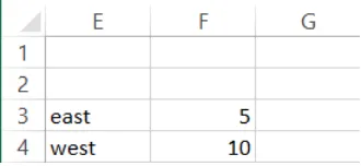
For example, suppose you want to name cell F3 east and cell F4 west. See Figure 1-2 and the

Eastwestempt.xlsx file. Select cell F3, type east in the Name box, and then press Enter. Select cell F4, type west in the Name box, and press Enter. If you now reference cell F3 in another cell, you see =east instead of =F3. This means that whenever you see the reference east in a formula, Excel will insert whatever is in cell F3.

FIGURE 1-2 Name cell F3 east and cell F4 west.

Suppose you want to assign a rectangular range of cells (such as A1:B4) the name Data. Select the cell range A1:B4, type Data in the Name box, and press Enter. Now a formula such as

(31)

Range names CHAPTER 1 3

FIGURE 1-3 Name the A1:B4 range Data.

Sometimes, you want to name a range of cells made up of several noncontiguous rectangular

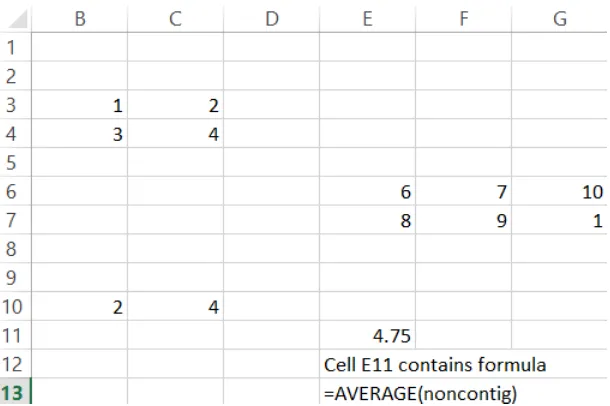
ranges. For example, in Figure 1-4 and the Noncontig.xlsx file, you might want to assign the name

Noncontig to the range consisting of cells B3:C4, E6:G7, and B10:C10. To assign this name, select any one of the three rectangles making up the range (B3:C4 for now). Hold down the Ctrl key and then select the other two ranges (E6:G7 and B10:C10). Now release the Ctrl key, type the name Noncontig

in the Name box, and press Enter. Using Noncontig in any formula will now refer to the contents of cells B3:C4, E6:G7, and B10:C10. For example, entering the formula =AVERAGE(Noncontig) in cell E11 yields 4.75 (because the 12 numbers in your range add up to 57, and 57/12 = 4.75).

(32)

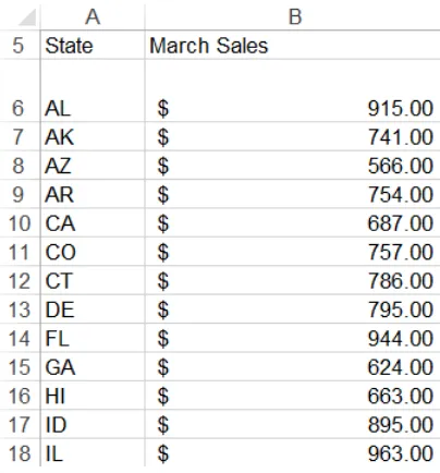
Creating named ranges by using Create From Selection

The Statestemp.xlsx worksheet contains sales during March for each of the 50 US states. Figure 1-5 shows a subset of this data. You would like to name each cell in the B6:B55 range with the cor-rect state abbreviation. To do this, select the A6:B55 range and click Create From Selection in the Defined Names group on the Formulas tab (see Figure 1-6) and then select the Left Column check box, as indicated in Figure 1-7.

FIGURE 1-5 By naming the cells that contain state sales with state abbreviations, you can use the abbreviation rather than the cell’s column letter and row number when you refer to the cell.

(33)

FIGURE 1-7 Select the Left Column check box.

Excel now knows to associate the names in the first column of the selected range with the cells in

the second column of the selected range. Thus, B6 is assigned the range name AL, B7 is named AK, and so on. Creating these range names in the Name box would have been incredibly tedious! Click the drop-down arrow in the Name box to verify that these range names have been created.

Creating range names by using Define Name

If you choose Name Manager on the Formulas tab and select Define Name from the menu shown

in Figure 1-6, the New Name dialog box shown in Figure 1-8 opens.

(34)

Suppose you want to assign the name range1 (range names are not case sensitive) to the cell range A2:B7. Type range1 in the Name box and then point to the range or type =A2:B7 in the Refers To

area. The New Name dialog box will now look like Figure 1-9. Click OK, and you’re done.

FIGURE 1-9 The New Name dialog box looks like this after creating a range name.

If you click the Scope arrow, you can select Workbook or any worksheet in your workbook. This decision is discussed later in this chapter, so for now, just choose the default scope of Workbook. You can also add comments for any of your range names.

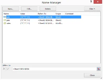
Name Manager

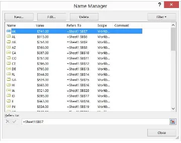
If you now click the Name arrow, the name range1 (and any other ranges you have created) appears in the Name box. In Excel 2013, there is an easy way to edit or delete your range names. Open Name Manager by selecting the Formulas tab and then click Name Manager from the menu shown in Figure 1-6. You now see a list of all range names. For example, for the States.xlsx file, the Name Manager dialog box will look like Figure 1-10.

To edit any range name, double-click the range name or select the range name and click Edit; you can then change the name of the range, the cells the range refers to, or the scope of the range.

To delete any subset of range names, first select the range names you want to delete. If the range names are listed consecutively, select the first range name in the group you want to delete, hold

down the Shift key, and select the last range name in the group. If the range names are not listed consecutively, you can select any range name you want to delete and then hold down the Ctrl key while you select the other range names for deletion. Then press the Delete key to delete the selected range names.

(35)

FIGURE 1-10 This is the Name Manager dialog box for States.xlsx.

Answers to this chapter’s questions

This section provides the answers to the questions that are listed at the beginning of the chapter.

I want the total sales in Arizona, California, Montana, New York, and New Jersey. Can I use a formula to compute the total sales in a form such as AZ+CA+MT+NY+NJ instead of SUM(A21:A25) and still get the right answer?

Return to the States.xlsx file, in which you assigned each state’s abbreviation as the range name for the state’s sales. If you want to compute total sales in Alabama, Alaska, Arizona, and Arkansas, clearly you could use the formula SUM(B6:B9). You could also point to cells B6, B7, B8, and B9, and the for-mula would be entered as =AL+AK+AZ+AR. The latter forfor-mula is self-describing.

As another illustration of how to use range names, look at the Historicalinvesttemp.xlsx file, shown in Figure 1-11, which contains annual percentage returns on stocks, T-bills, and bonds. (Some rows are

(36)

FIGURE 1-11 This figure shows historical investment data.

Select the B8:D89 cell range and then choose Formulas and Create From Selection. For this example, names are created in the top row of the range. The B8:B89 range is named Stocks, the C8:C89 range T.Bills, and the D8:D89 range T.Bonds. Now you no longer need to remember where your data is. For example, in cell B91, after typing =AVERAGE(, you can press F3, and the Paste Name dialog box opens, as shown in Figure 1-12. You can also bring up a list of range names that can be pasted in formulas if you start typing and click Use InFormula on the Formulas tab.

(37)

You can select Stocks in the Paste Name list and click OK. After entering the closing parenthesis, the formula, =AVERAGE(Stocks), computes the average return on stocks (11.28 percent). The beauty of this approach is that even if you don’t remember where the data is, you can work with the stock return data anywhere in the workbook!

This chapter would be remiss if it did not mention the exciting AutoComplete capabilities of Excel 2013. If you begin typing =Average(T, Excel shows you a list of range names and functions that begin with T, and you can just double-click T.Bills to complete the entry of the range name.

What does a formula such as Average(A:A) do?

If you use a column name (in the form of A:A, C:C, and so on) in a formula, Excel treats an entire column as a named range. For example, entering the =AVERAGE(A:A) formula averages all numbers in column A. Using a range name for an entire column is very helpful if you frequently enter new data in a column. For example, if column A contains monthly sales of a product, as new sales data are entered each month, your formula computes an up-to-date monthly sales average. Use caution, however, because if you enter the =AVERAGE(A:A) formula in column A, you will get a circular reference mes-sage because the value of the cell containing the average formula depends on the cell containing the average. You learn how to resolve circular references in Chapter 10, “Circular references.” Similarly, entering the =AVERAGE(1:1) formula averages all numbers in row 1.

What is the difference between a name with workbook scope and one with worksheet scope?

The Sheetnames.xlsx file will help you understand the difference between range names that have

workbook scope and range names that have worksheet scope. When you create names with the Name box, the names default to workbook scope. For example, suppose you use the Name box to assign the name sales to the cell range E4:E6 in Sheet3, and these cells contain the numbers 1, 2, and 4, respectively. If you enter a formula such as =SUM(sales) in any worksheet, you obtain an answer of 7 because the Name box creates names with workbook scope, so anywhere in the workbook you refer to the name sales (which has workbook scope), the name refers to cells E4:E6 of Sheet3. In any worksheet, if you now enter the =SUM(sales) formula, you will obtain 7 because anywhere in the workbook, Excel links sales to cells E4:E6 of Sheet3.

Now suppose that you type 4, 5, and 6 in cells E4:E6 of Sheet1 and 3, 4, and 5 in cells E4:E6 of Sheet2, and then you open Name Manager, give the name jam to cells E4:E6 of Sheet1, and define the

scope of this name as Sheet1. Then you move to Sheet2, open Name Manager, give the name jam to

(38)

FIGURE 1-13 The Name Manager dialog box displays worksheet and workbook names.

Now, what if you enter the =SUM(jam) formula in each sheet? In Sheet 1, =SUM(jam) will total cells E4:E6 of Sheet1. Because those cells contain 4, 5, and 6, you obtain 15. In Sheet2, =SUM(jam) will total cells E4:E6 of Sheet2, yielding 3 + 4 + 5 = 12. In Sheet3, however, the =SUM(jam) formula will yield a #NAME? error because no range is named jam in Sheet3. If you enter the =SUM(Sheet2!jam) formula anywhere in Sheet3, Excel will recognize the worksheet-level name that represents cell range E4:E6 of Sheet2 and yield a result of 3 + 4 + 5 = 12. Thus, by prefacing a worksheet-level name by its sheet name followed by an exclamation point (!), you can refer to a worksheet-level range in a worksheet

other than the sheet in which the range is defined.

I really am getting to like range names. I have started defining range names for many of the workbooks I have developed at the office. However, the range names do not show up in my formulas. How can I make recently created range names show up in previously created formulas?

(39)

FIGURE 1-14 This figure shows how to apply range names to formulas.

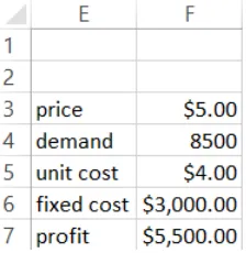
The price of a product was entered in cell F3 and product demand of =10000–300*F3 in cell F4.

The unit cost and fixed cost are entered in cells F5 and F6, respectively, and profit is computed in cell

F7 with the =F4*(F3–F5)–F6 formula. In this example, Formulas, Create From Selection, and then

Left Column are used to name cell F3 price, cell F4 demand, cell F5 unit cost, cell F6 fixed cost, and cell F7 profit. You would like these range names to show up in the cell F4 and cell F7 formulas. To apply

the range names, first select the range where you want the range names applied (in this case, F4:F7).

Now open the Defined Names group on the Formulas tab, click the Define Name arrow, and then

choose Apply Names. Highlight the names you want to apply and then click OK. Note that cell F4 now contains the =10000–300*price formula, and cell F7 contains the =demand*(price–unit_cost)–

fixed_cost formula, as you wanted.

By the way, if you want the range names to apply to the entire worksheet, select the entire work-sheet by clicking the Select All button at the intersection of the column and row headings.

How can I paste a list of all range names (and the cells they represent) into my worksheet?

Press F3 to open the Paste Name box and then click the Paste List button. (See Figure 1-12.) A list of range names and the cells each corresponds to will be pasted into your worksheet, beginning at the current cell location.

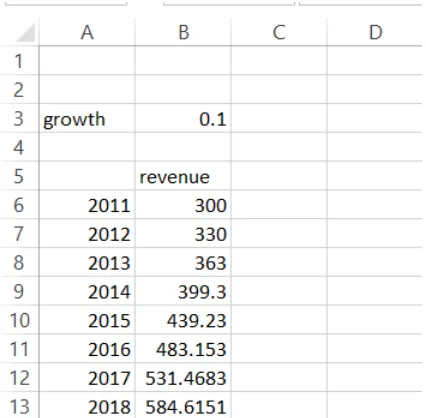
I am computing projected annual revenues as a multiple of last year’s revenue. Is there a way to have the formula look like (1+growth)*last year?

(40)

FIGURE 1-15 Create a range name for the previous year.

To begin, use the Name box to name cell B3 growth. Now comes the good part! Move the cursor to B7 and open the New Name dialog box by clicking Define Name in the Defined Names group

on the Formulas tab. Fill in the New Name dialog box as shown in Figure 1-16.

FIGURE 1-16 In any cell, this name refers to the cell above the active cell.

(41)

range, each cell will contain the formula you want and will multiply 1.1 by the contents of the cell directly above the active cell.

For each day of the week, we are given the hourly wage and hours worked. Can we compute total salary for each day with the wages*hours formula?

As shown in Figure 1-17 (see the Namedrows.xlsx file), row 12 contains daily wage rates, and row 13

contains hours worked each day.

FIGURE 1-17 In any cell, this name refers to the cell above the active cell.

You can select row 12 (by clicking the 12) and use the Name box to enter the name wage. Select row 13 and type the name hours in the Name box. If you now enter the wage*hours formula in cell

F14 and copy this formula to the G14:L14 range, you can see that Excel finds the wage and hour val -ues and multiplies them in each column.

Remarks

■ Excel does not allow you to use the letters r and c as range names.

■ The only symbols allowed in range names are periods (.) and underscores (_).

■ If you use Create From Selection to create a range name, and your name contains spaces, Excel inserts an underscore (_) to fill in the spaces. For example, Product 1 is created as Product_1.

■ Range names cannot begin with numbers or look like a cell reference. For example, 3Q and A4 are not allowed as range names. Because Excel 2013 has more than 16,000 columns, a range name such as cat1 is not permitted because there is a CAT1 cell. If you try to name a cell CAT1, Excel tells you the name is invalid. Probably your best alternative is to name the cell cat1_.

Problems

1. The Stock.xlsx file contains monthly stock returns for General Motors and Microsoft. Name the ranges containing the monthly returns for each stock and compute the average monthly return on each stock.

(42)

3. In cells Q5 and Q6 in the Citydistances.xlsx file, you can enter the latitude and longitude of any city and, in Q7 and Q8, the latitude and longitude of a second city. Cell Q10 computes the

distance between the two cities. Define range names for the latitude and longitude of each

city and ensure that these names show up in the formula for total distance.

4. The Sharedata.xlsx file contains the numbers of shares you own of each stock and the price of each stock. Compute the value of the shares of each stock with the shares*price formula.

5. Create a range name that averages the past five years of sales data. Assume annual sales are

(43)

15

C H A P T E R 2

Lookup functions

Questions answered in this chapter:

■ How can I write a formula to compute tax rates based on income? ■ Given a product ID, how can I look up the product’s price?

■ Suppose that a product’s price changes over time. I know the date the product was sold. How can I write a formula to compute the product’s price?

Syntax of the lookup functions

Lookup functions enable you to look up values from worksheet ranges. In Microsoft Excel 2013, you can perform both vertical lookups (by using the VLOOKUP function) and horizontal lookups (by using the HLOOKUP function). In a vertical lookup, the lookup operation starts in the first column of a worksheet range. In a horizontal lookup, the operation starts in the first row of a worksheet range. Because the majority of formulas using lookup functions involve vertical lookups, this chapter con-centrates on VLOOKUP functions.

VLOOKUp syntax

The syntax of the VLOOKUP function is as follows. The brackets ([ ]) indicate optional arguments.

VLOOKUP(lookup value,table range,column index,[range lookup])

■ Lookup value is the value you want to look up in the first column of the table range. ■ Table range is the range that contains the entire lookup table. The table range includes the

first column, in which you try to match the lookup value, and any other columns in which you

want to look up formula results.

■ Column index is the column number in the table range from which the value of the lookup function is obtained.

■ Range lookup is an optional argument. The point of range lookup is to specify an exact or approximate match. If the range lookup argument is True or omitted, the first column of the

table range must be in ascending numerical order. If the range lookup argument is True or

(44)

16 CHAPTER 2 Lookup functions

range, Excel bases the lookup on the row of the table in which the exact match is found. If the

range lookup argument is True or omitted and an exact match does not exist, Excel bases the

lookup on the largest value in the first column that is less than the lookup value. If the range lookup argument is False and an exact match to the lookup value is found in the first column

of the table range, Excel bases the lookup on the row of the table in which the exact match is found. If no exact match is obtained, Excel returns an #N/A (Not Available) response. Note that a range lookup argument of 1 is equivalent to True, whereas a range lookup argument of

0 is equivalent to False.

hLOOKUp syntax

In an HLOOKUP function, Excel tries to locate the lookup value in the first row (not the first column)

of the table range. For an HLOOKUP function, use the VLOOKUP syntax and change column to row.

Now, explore some interesting examples of lookup functions.

Answers to this chapter’s questions

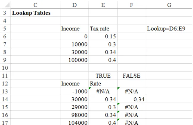
How can I write a formula to compute tax rates based on income?

The following example shows how a VLOOKUP function works when the first column of the table

range consists of numbers in ascending order. Suppose that the tax rate depends on income, as shown in Table 2-1.

TABLE 2-1 Tax rate on income

Income level Tax rate

$0–$9,999 15%

$10,000–$29,999 30%

$30,000–$99,999 34%

$100,000 and over 40%

To see an example of how to write a formula that computes the tax rate for any income level, open

(45)

Lookup functions CHAPTER 2 17

FIGURE 2-1 Use a lookup function to compute a tax rate. The numbers in the first column of the table range are sorted in ascending order.

First, the relevant information (tax rates and break points) was entered in cell range D6:E9. The table range is named D6:E9 lookup. It’s recommended always to name the cells you’re using as the table range. If you do so, you need not remember the exact location of the table range, and when you copy any formula involving a lookup function, the lookup range will always be correct. To illus-trate how the lookup function works, some incomes were entered in the D13:D17 range. By copying the VLOOKUP(D13,Lookup,2,True) formula from E13 to E14:E17, the tax rate was computed for the income levels listed in D13:D17. Examine how the lookup function worked in cells E13:E17. Note that because the column index in the formula is 2, the answer always comes from the second column of the table range.

■ In D13, the income of –$1,000 yields #N/A because –$1,000 is less than the lowest income

level in the first column of the table range. If you want a tax rate of 15 percent associated with

an income of –$1,000, replace the 0 in D6 with a number that is –1,000 or smaller.

■ In D14, the income of $30,000 exactly matches a value in the first column of the table range, so the function returns a tax rate of 34 percent.

■ In D15, the income level of $29,000 does not exactly match a value in the first column of the table range, which means the lookup function stops at the largest number less than $29,000

in the first column of the range—$10,000 in this case. This function returns the tax rate in

(46)

■ In D16, the income level of $98,000 does not yield an exact match in the first column of the

table range. The lookup function stops at the largest number less than $98,000 in the first

column of the table range. This returns the tax rate in column 2 of the table range opposite

$30,000—34 percent.

■ In D17, the income level of $104,000 does not yield an exact match in the first column of the

table range. The lookup function stops at the largest number less than $104,000 in the first

column of the table range, which returns the tax rate in column 2 of the table range opposite

$100,000—40 percent.

In F13:F17, the value of the range lookup argument was changed from True to False, and the VLOOKUP(D13,Lookup,2,False) formula was copied from F13 to F14:F17. Cell F14 still yields a 34

percent tax rate because the first column of the table range contains an exact match to $30,000. All

the other entries in F13:F17 display #N/A because none of the other incomes in D13:D17 has an exact

match in the first column of the table range.

Given a product ID, how can I look up the product’s price?

Often, the first column of a table range does not consist of numbers in ascending order. For example,

the first column of the table range might list product ID codes or employee names. In my experience teaching thousands of financial analysts, I’ve found that many people don’t know how to deal with lookup functions when the first column of the table range does not consist of numbers in ascending

order. In these situations, remember only one simple rule: Use False as the value of the range lookup

argument.

Here’s an example. In the Lookup.xlsx file (see Figure 2-2), you can see the prices for five products,

listed by their product ID code. How do you write a formula that takes a product ID code and returns the product price?

FIGURE 2-2 Look up prices from product ID codes. When the table range isn’t sorted in ascending order, enter

False as the last argument in the lookup function formula.

(47)

Because the product IDs in the Lookup2 (H11:I15) table range are not listed in alphabetical order, an incorrect price ($3.50) is returned. If you enter the VLOOKUP(H18,Lookup2,2,False) formula in cell I18,

the correct price ($5.20) is returned.

You would also use False in a formula designed to find an employee’s salary by using the employ -ee’s last name or ID number.

By the way, you can see in Figure 2-2 that columns A to G are hidden. To hide columns, you begin by selecting the columns you want to hide. Click the Home tab on the ribbon. In the Cells group, choose Format, point to Hide & Unhide (under Visibility), and then choose Hide Columns.

Suppose that a product’s price changes over time. I know the date the product was sold. How can I write a formula to compute the product’s price?

Suppose the price of a product depends on the date the product was sold. How can you use a lookup

function in a formula that will pick up the correct product price? More specifically, suppose the price

of a product is as shown in the following table:

Date sold Price

January–April 2005 $98

May–July 2005 $105

August–December 2005 $112

Write a formula to determine the correct product price for any date on which the product is sold in the year 2005. For variety, use an HLOOKUP function. The dates when the price changes are in the

first row of the table range. See the Datelookup.xlsx file, shown in Figure 2-3.

FIGURE 2-3 Use an HLOOKUP function to determine a price that changes depending on the date it’s sold.

The HLOOKUP(B8,lookup,2,TRUE) formula is copied from C8 to C9:C11. This formula tries to match

the dates in column B with the first row of the B2:D3 range. At any date between 1/1/05 and 4/30/05,

(48)

7/31/05, the lookup stops at 5/1/05 and returns the price in C3; and for any date later than 8/1/05, the lookup stops at 8/1/05 and returns the price in D3.

Problems

1. The Hr.xlsx file gives employee ID codes, salaries, and years of experience. Write a formula that yields the employee’s salary from a given ID code. Write another formula that yields the employee’s years of experience from a given ID code.

2. The Assign.xlsx file gives the assignment of workers to four groups. The suitability of each worker for each group (on a scale from 0 to 10) is also given. Write a formula that gives the suitability of each worker for the group to which the worker is assigned.

3. _{You are thinking of advertising Microsoft products on a sports telecast. As you buy more ads,} the price of each ad decreases as shown in the following table:

Number of ads Price per ad per ad. Write a formula that yields the total cost of purchasing any number of ads.

4. _{You are thinking of advertising Microsoft products on a popular TV music program. You pay}

one price for the first group of ads, but as you buy more ads, the price per ad decreases as

shown in the following table:

For example, if you buy 8 ads, you pay $12,000 per ad for the first 5 ads and $11,000 for each of the next 3 ads. If you buy 14 ads, you pay $12,000 for each of the first 5 ads, $11,000 for

(49)

5. _{The annual rate your bank charges you to borrow money for 1, 5, 10, or 30 years is shown in} the following table:

If you borrow money from the bank for any duration from 1 through 30 years that’s not listed in the table, your rate is found by interpolating between the rates given in the table. For example, you borrow money for 15 years. Because 15 years is one quarter of the way between 10 years and 30 years, the annual loan rate would be calculated as follows:

Write a formula that returns the annual interest rate on a loan for any period between 1 and 30 years.

6. _{The distance between any two US cities (excluding cities in Alaska and Hawaii) can be} approxi-mated by this formula:

69 * (lat1 - lat2)2 _{+ (long1 - long2)}2

The Citydata.xlsx file contains the latitude and longitude of selected US cities. Create a table

that gives the distance between any two of the listed cities.

7. In the Pinevalley.xlsx file, the first worksheet contains the salaries of several employees at Pine Valley University, the second worksheet contains the age of the employees, and the third worksheet contains the years of experience. Create a fourth worksheet that contains the sal-ary, age, and experience for each employee.

8. The Lookupmultiplecolumns.xlsx file contains information about several sales made at an electronics store. A salesperson’s name will be entered in B17. Write an Excel formula that can be copied from C17 to D17:F17 that extracts each salesperson’s radio sales to C17, TV sales to D17, printer sales to E17, and CD sales to F17.

+ = 4

1₍₉₎ 4

(50)

9. The Grades.xlsx file contains students’ grades on an exam. Suppose the curve is as follows:

Score Grade

Below 60 F

60–69 D

70–79 C

80–89 B

90 and above A

Use Excel to return each student’s letter grade on this exam.

10. The Employees.xlsx file contains the ranking each of 35 workers has given (on a 0–10 scale) to

three jobs. The file also gives the job to which each worker is assigned. Use a formula to com -pute each worker’s ranking for the job to which the worker is assigned.

(51)

23

C H A P T E R 3

INDEX function

Questions answered in this chapter:

■ I have a list of distances between US cities. How can I write a function that returns the distance between, for example, Seattle and Miami?

■ Can I write a formula that references the entire column containing the distances between each city and Seattle?

Syntax of the

INDEX

function

The INDEX function enables you to return the entry in any row and column within an array of num-bers. The most commonly used syntax for the INDEX function is the following:

INDEX(Array,Row Number,Column Number)

To illustrate, the INDEX(A1:D12,2,3) formula returns the entry in the second row and third column of the A1:D12 array. This entry is the one in cell C2.

Answers to this chapter’s questions

I have a list of distances between US cities. How can I write a function that returns the dis-tance between, for example, Seattle and Miami?

(52)

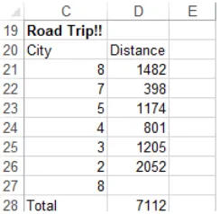
24 CHAPTER 3 INDEX function

FIGURE 3-1 You can use the INDEX function to calculate the distance between cities.

Suppose that you want to enter the distance between Boston and Denver in a cell. Because

dis-tances from Boston are listed in the first row of the array named Distances, and distances to Denver are listed in the fourth column of the array, the appropriate formula is INDEX(distances,1,4). The

results show that Boston and Denver are 1,991 miles apart. Similarly, to find the (much longer) dis -tance between Seattle and Miami, you would use the INDEX(dis-tances,6,8) formula. Seattle and Miami are 3,389 miles apart.

Imagine that a resident of Seattle, Kurt Sovain is embarking on a road trip to visit relatives in Phoenix, Los Angeles (USC!), Denver, Dallas, and Chicago. At the conclusion of the road trip, Kurt returns to Seattle. Can you easily compute how many miles Kurt travels on the trip? As you can see in Figure 3-2, you simply list the cities Kurt visited (8-7-5-4-3-2-8) in the order he visited them, starting and ending in Seattle, and copy the INDEX(distances,C21,C22) formula from D21 to D26. The formula in D21 computes the distance between Seattle and Phoenix (city number 7), the formula in D22 com-putes the distance between Phoenix and Los Angeles, and so on. Kurt will travel a total of 7,112 miles on his road trip. Just for fun, use the INDEX function to show that the Miami Heat travel more miles during the NBA season than any other team.