PUBLISHED BY Microsoft Press
A Division of Microsoft Corporation One Microsoft Way
Redmond, Washington 98052-6399 Copyright © 2010 by Curtis Frye
All rights reserved. No part of the contents of this book may be reproduced or transmitted in any form or by any means without the written permission of the publisher.
Library of Congress Control Number: 2010924442
Printed and bound in the United States of America.
1 2 3 4 5 6 7 8 9 QWT 5 4 3 2 1 0
A CIP catalogue record for this book is available from the British Library.
Microsoft Press books are available through booksellers and distributors worldwide. For further infor mation about international editions, contact your local Microsoft Corporation office or contact Microsoft Press International directly at fax (425) 936-7329. Visit our Web site at www.microsoft.com/mspress. Send comments to mspinput@ microsoft.com.
Microsoft, Microsoft Press, Access, Encarta, Excel, Fluent, Internet Explorer, MS, Outlook, PivotChart, PivotTable, PowerPoint, SmartArt, SQL Server, Visual Basic, Windows and Windows Mobile are either registered trademarks or trademarks of the Microsoft group of companies. Other product and company names mentioned herein may be the trademarks of their respective owners.
The example companies, organizations, products, domain names, e-mail addresses, logos, people, places, and events depicted herein are fictitious. No association with any real company, organization, product, domain name, e-mail address, logo, person, place, or event is intended or should be inferred.
This book expresses the author’s views and opinions. The information contained in this book is provided without any express, statutory, or implied warranties. Neither the authors, Microsoft Corporation, nor its resellers, or distributors will be held liable for any damages caused or alleged to be caused either directly or indirectly by this book.
Acquisitions Editor: Juliana Aldous Developmental Editor: Devon Musgrave Project Editor: Valerie Woolley
Editorial Production: Online Training Solutions, Inc.
Technical Reviewer: Bob Dean; Technical Review services provided by Content Master, a member of CM Group, Ltd.
iii
What do you think of this book? We want to hear from you! Microsoft is interested in hearing your feedback so we can continually improve our books and learning resources for you. To participate in a brief online survey, please visit: microsoft.com/learning/booksurvey
iv Contents
3 Performing Calculations on Data
55
Naming Groups of Data . . . .56
Creating Formulas to Calculate Values. . . .60
Summarizing Data That Meets Specific Conditions. . . 70
Finding and Correcting Errors in Calculations . . . 74
Key Points . . . 81
4 Changing Workbook Appearance
83
Formatting Cells. . . .845 Focusing on Specific Data by Using Filters
121
Limiting Data That Appears on Your Screen. . . .1226 Reordering and Summarizing Data
143
Sorting Worksheet Data. . . .144Organizing Data into Levels. . . .153
Looking Up Information in a Worksheet. . . .160
Key Points . . . .165
7 Combining Data from Multiple Sources
167
Using Workbooks as Templates for Other Workbooks. . . .168Linking to Data in Other Worksheets and Workbooks . . . 175
Consolidating Multiple Sets of Data into a Single Workbook . . . .180
Grouping Multiple Sets of Data . . . .184
Contents v
8 Analyzing Alternative Data Sets
189
Defining an Alternative Data Set . . . .1909 Creating Dynamic Worksheets by Using PivotTables
211
Analyzing Data Dynamically by Using PivotTables . . . .212vi Contents
12 Automating Repetitive Tasks by Using Macros
329
Enabling and Examining Macros. . . .330
13 Working with Other Microsoft Office Programs
349
Including Office Documents in Workbooks . . . .350Storing Workbooks as Parts of Other Office Documents. . . 355
Creating Hyperlinks. . . .358
Pasting Charts into Other Documents . . . .364
Key Points . . . .365
14 Collaborating with Colleagues
367
Sharing Workbooks. . . .368What do you think of this book? We want to hear from you!
Microsoft is interested in hearing your feedback so we can continually improve our books and learning resources for you. To participate in a brief online survey, please visit:
vii
Acknowledgments
Creating a book is a time-consuming (sometimes all-consuming) process, but working within an established relationship makes everything go much more smoothly. In that light, I’d like to thank Juliana Aldous Atkinson and Devon Musgrave from Microsoft Press for bringing me back for another tilt at the windmill. I’ve been lucky to work with Microsoft Press for the past nine years, and always enjoy working with Valerie Woolley, who oversaw this project for Microsoft Press.
I’d also like to thank Kathy Krause and Marlene Lambert of OTSI. Kathy provided able project oversight and a thorough copy edit, while Marlene managed the production process. Bob Dean did a great job with the technical edit, Elisabeth Van Every brought everything together as the book’s compositor, and Jaime Odell completed the project with a careful proofread. I hope I get the chance to work with all of them again.
ix
Introducing Microsoft Excel 2010
For those of you who are upgrading to Microsoft Excel 2010 from an earlier version of the program, this introduction summarizes the new features in Excel 2010. One of the first things you’ll notice about Excel 2010 is that the program incorporates the ribbon, which was introduced in Excel 2007. If you used Excel 2003 or an earlier ver-sion of Excel, you’ll need to spend only a little bit of time working with the new user interface to bring yourself back up to your usual proficiency.Managing Excel Files and Settings
in the Backstage View
If you used Excel 2007, you’ll immediately notice one significant change: the Microsoft Office button, located at the top left corner of the program window in Excel 2007, has been replaced by the File tab. After releasing the 2007 Microsoft Office System, the Office User Experience team re-examined the programs’ user interfaces to determine how they could be improved. During this process, they discovered that it was possible to divide user tasks into two categories: “in” tasks, such as formatting and formula creation, which affect the contents of the workbook directly, and “out” tasks, such as saving and printing, which could be considered workbook management tasks. When the User Experience and Excel teams focused on the Excel 2007 user interface, they discovered that several workbook management tasks were sprinkled among the ribbon tabs that contained content-related tasks. The Excel team moved all of the workbook management tasks to the File tab, which users can click to display these commands in the new Backstage view. Introducing Microsoft Excel 2010 . . . ixManaging Excel Files and Settings in the Backstage View. . . .ix
Managing Large Worksheets by Using the 64-bit Version of Excel 2010 . . . xxii
x Introducing Microsoft Excel 2010
Previewing Data by Using Paste Preview
Introducing Microsoft Excel 2010 xi
In Excel 2010, you can take advantage of the new Paste Preview capability to see how your data will appear in the worksheet before you commit to the paste. By pointing to any of the icons in the Paste Options palette, you can switch between options to discover the one that makes your pasted data appear the way you want it to.
Troubleshooting The appearance of buttons and groups on the ribbon changes depending on the width of the program window. For information about changing the appearance of the ribbon to match our screen images, see “Modifying the Display of the Ribbon” at the beginning of this book.
Customizing the Excel 2010 User Interface
xii Introducing Microsoft Excel 2010
Summarizing Data by Using More Accurate
Functions
In earlier versions of Excel, the program contained statistical, scientific, engineering, and financial functions that would return inaccurate results in some relatively rare circumstances. For Excel 2010, the Excel programming team identified the functions that returned inaccurate results and collaborated with academic and industry analysts to improve the functions’ accuracy.
The Excel team also changed the naming conventions used to identify the program’s functions. This change is most noticeable with regard to the program’s statistical func-tions. The table below lists the statistical distribution functions that have been improved in Excel 2010.
Distribution Functions
Beta BETA.DIST, BETA.INV Binomial BINOM.DIST, BINOM.INV
Chi squared CHISQ.DIST, CHISQ.DIST.RT, CHISQ.INV, CHISQ.INV.RT Exponential EXPON.DIST
Introducing Microsoft Excel 2010 xiii
Student’s t T.DIST, T.DIST.RT, T.DIST.2T, T.INV, T.INV.2T
Weibull WEIBULL.DIST
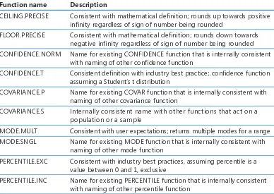
Excel 2010 also contains more accurate statistical summary and test functions. The following table lists those functions, as well as the new naming convention that distinguishes between new and old functions. The Excel programming team chose to retain the older functions to ensure that workbooks created in Excel 2010 would be compatible with workbooks created in previous versions of the program.
Function name Description
CEILING.PRECISE Consistent with mathematical definition; rounds up towards positive infinity regardless of sign of number being rounded
FLOOR.PRECISE Consistent with mathematical definition; rounds down towards negative infinity regardless of sign of number being rounded CONFIDENCE.NORM Name for existing CONFIDENCE function that is internally consistent
with naming of other confidence function
CONFIDENCE.T Consistent definition with industry best practice;. confidence function assuming a Student’s t distribution
COVARIANCE.P Name for existing COVAR function that is internally consistent with naming of other covariance function
COVARIANCE.S Internally consistent name with other functions that act on a population or a sample
MODE.MULT Consistent with user expectations; returns multiple modes for a range MODE.SNGL Name for existing MODE function that is internally consistent with
naming of other mode function
PERCENTILE.EXC Consistent with industry best practices, assuming percentile is a value between 0 and 1, exclusive
xiv Introducing Microsoft Excel 2010
Function name Description
PERCENTRANK.EXC Consistent with industry best practices; assuming percentile is a value between 0 and 1, exclusive
PERCENTRANK.INC Name for existing PERCENTRANK function that is internally consistent with naming of other PERCENTRANK function
QUARTILE.EXC Consistent with industry best practices, assuming percentile is a value between 0 and 1, exclusive
QUARTILE.INC Name for existing QUARTILE function that is internally consistent with naming of other quartile function
RANK.AVG Consistent with industry best practices, returning the average rank when there is a tie
RANK.EQ Name for existing RANK function that is internally consistent with naming of other rank function
STDEV.P Name for existing STDEVP function that is internally consistent with naming of other standard deviation function
STDEV.S Name for existing STDEV function that is internally consistent with naming of other standard deviation function
VAR.P Name for existing VARP function that is internally consistent with naming of other variance function
VAR.S Name for existing VAR function that is internally consistent with naming of other variance function
CHISQ.TEST Name for existing CHITEST function that is internally consistent with naming of other hypothesis test functions
F.TEST Name for existing FTEST function that is internally consistent with naming of other hypothesis functions
T.TEST Name for existing TTEST function that is internally consistent with naming of other hypothesis functions
Z.TEST Name for existing ZTEST function that is internally consistent with naming of other hypothesis functions
Introducing Microsoft Excel 2010 xv
When a user saves a workbook that contains functions that are new in Excel 2010 to an older format, the Compatibility Checker flags the functions and indicates that they will return a #NAME? error when the workbook is opened in Excel 2007 or earlier versions.
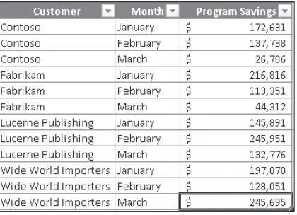
Summarizing Data by Using Sparklines
In his book Beautiful Evidence, Edward Tufte describes sparklines as “intense, simple, wordlike graphics.” In Excel 2010, sparklines take the form of small charts that summarize data in a single cell. These small but powerful additions to Excel 2010 enhance the program’s reporting and summary capabilities.
xvi Introducing Microsoft Excel 2010
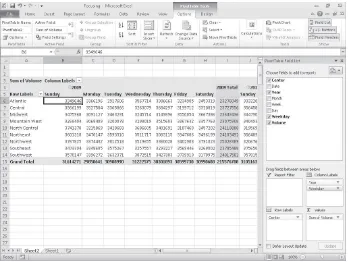
Filtering PivotTable Data by Using Slicers
With PivotTables, users can summarize large data sets efficiently, such as by rearranging values dynamically to emphasize different aspects of the data. It’s often useful to be able to limit the data that appears in a PivotTable, so the Excel team included the functionality for users to filter PivotTables. The PivotTable indicates that a filter is present for a particular data column, but it doesn’t indicate which items are currently displayed or hidden by the filter.
Introducing Microsoft Excel 2010 xvii
Filtering PivotTable Data by Using Search Filters
xviii Introducing Microsoft Excel 2010
Visualizing Data by Using Improved Conditional
Formats
In Excel 2007, the Excel programming team greatly improved the user’s ability to change a cell’s format based on the cell’s contents. One new conditional format, data bars, indicated a cell’s relative value by the length of the bar within the cell that contained the value. The cell in the range that contained the smallest value displayed a zero-length bar, and the cell that contained the largest value displayed a bar that spanned the entire cell width.
Introducing Microsoft Excel 2010 xix
representing negative values extend to the left of the baseline, not to the right. In Excel 2007, the conditional formatting engine placed the zero-length data bar in the cell that con-tained the smallest value, regardless of whether that value was positive or negative. You have much more control over your data bars’ formatting in Excel 2010 than in Excel 2007. When you create a data bar in Excel 2010, it has a solid color fill, not a gradient fill like the bars in Excel 2007. The gradient fill meant that the color of the Excel 2007 data bars faded as the bar extended to the right, making the cells’ relative values harder to discern. In Excel 2010 you can select a solid or gradient fill style, apply borders to data bars, and change the fill and border colors for both positive and negative values.
xx Introducing Microsoft Excel 2010
Introducing Microsoft Excel 2010 xxi
Creating and Displaying Math Equations
Scientists and engineers who use Microsoft Excel to support their work often want to include equations in their workbooks to help explain how they arrived at their results. Excel 2010 includes an updated equation designer with which you can create any equation you require. The new editor has several common equations built in, such as the quadratic formula and the Pythagorean theorem, but it also contains numerous templates that you can use to create custom equations quickly.
Editing Pictures within Excel 2010
When you present data in an Excel workbook, you can insert images into your work-sheets to illustrate aspects of your data. For example, a shipping company could display a scanned image of a tracking label or a properly prepared package. Rather than having to edit your images in a separate program and then insert them into your Excel 2010 workbook, you can insert the image and then modify it by using the editing tools built into Excel 2010.
xxii Introducing Microsoft Excel 2010
Managing Large Worksheets by Using the 64-bit
Version of Excel 2010
Some Excel 2010 users, such as business analysts and scientists, will need to manipulate extremely large data sets. In some cases, these data sets won’t fit into the more than one million rows available in a standard Excel 2010 worksheet. To meet the needs of these users, the Excel product team developed the 64-bit version of Excel 2010. The 64-bit version takes advantage of the greater amount of random access memory (RAM) avail-able in newer computers. As a result of its ability to use more RAM than the standard 32-bit version of Excel 2010, users of the 64-bit version can store hundreds of millions of rows of data in a worksheet. In addition, the 64-bit version takes advantage of multi-core processors to manage its larger data collections efficiently.
All of the techniques described in Microsoft Excel 2010 Step by Step apply to both the 32-bit and 64-bit versions of the program.
Summarizing Large Data Sets by Using the
PowerPivot (Project Gemini) Add-In
As businesses collect and maintain increasingly large data sets, the need to analyze that data efficiently grows in importance. More powerful computers offer some performance improvements, but even the fastest computer takes a long time to process huge data sets when using traditional data-handling procedures. A new add-in, PowerPivot for Excel 2010, uses enhanced data management techniques to store the data in a computer’s memory, rather than forcing the Excel program to read the data from a hard disk. Reading data from a computer’s memory instead of a hard disk speeds up the data analysis and display operations substantially. Tasks that might have taken minutes to complete in Excel 2010 without the PowerPivot add-in now take seconds.
Introducing Microsoft Excel 2010 xxiii
Accessing Your Data from Almost Anywhere by
Using the Excel Web App and Excel Mobile 2010
As the workforce becomes increasingly mobile, information workers need to access their Excel 2010 data as they move around the world. To enable these mobile use scenarios, the Excel product team developed the Excel Web App and Excel Mobile 2010. The Excel Web App provides a high-fidelity experience that is very similar to the experience of using the Excel 2010 desktop application. In addition, you can collaborate with other users in real time. The Excel Web App identifies which changes were made by which users and enables you to decide which changes to keep and which to reject.
You can use the Excel Web App in Windows Internet Explorer 7 or 8, Safari 4, and Firefox 3.5.
With Excel Mobile 2010, you can access and, in some cases, manipulate your data by using a Windows Phone or other mobile device. If you have a Windows Phone running Windows Mobile 6.5, you can use Excel Mobile 2010 to view and edit your Excel 2010 workbooks. If you have another mobile device that provides access to the Web, you can use your device’s built-in Web browser to view your files.
xxv
Modifying the Display of the Ribbon
The goal of the Microsoft Office working environment is to make working with Office docu-ments, including Microsoft Word docudocu-ments, Excel workbooks, PowerPoint presentations, Outlook e-mail messages, and Access database tables, as intuitive as possible. You work with an Office document and its contents by giving commands to the program in which the document is open. All Office 2010 programs organize commands on a horizontal bar called the ribbon, which appears across the top of each program window whether or not there is an active document.
Ribbon tabs Ribbon groups
Commands are organized on task-specific tabs of the ribbon, and in feature-specific groups on each tab. Commands generally take the form of buttons and lists. Some appear in galleries. Some groups have related dialog boxes or task panes that contain additional commands.
Throughout this book, we discuss the commands and ribbon elements associated with the program feature being discussed. In this topic, we discuss the general appearance of the ribbon, things that affect its appearance, and ways of locating commands that aren’t visible on compact views of the ribbon.
Tip Some older commands no longer appear on the ribbon, but are still available in the program. You can make these commands available by adding them to the Quick Access Toolbar. For more information, see “Customizing the Excel 2010 Program Window” in Chapter 1, “Setting Up a Workbook.”
Dynamic Ribbon Elements
The ribbon is dynamic, meaning that the appearance of commands on the ribbon changes as the width of the ribbon changes. A command might be displayed on the ribbon in the form of a large button, a small button, a small labeled button, or a list entry. As the width of the ribbon decreases, the size, shape, and presence of buttons on the ribbon adapt to the available space.
Modifying the Display of the Ribbon . . . xxv
xxvi Modifying the Display of the Ribbon
For example, when sufficient horizontal space is available, the buttons on the Review tab of the Word program window are spread out and you’re able to see more of the commands available in each group.
Drop-down list
Small labeled button
Large button
If you decrease the width of the ribbon, small button labels disappear and entire groups of buttons hide under one button that represents the group. Click the group button to display a list of the commands available in that group.
Group button Small unlabeled buttons
When the window becomes too narrow to display all the groups, a scroll arrow appears at its right end. Click the scroll arrow to display hidden groups.
Scroll arrow
Changing the Width of the Ribbon
The width of the ribbon is dependent on the horizontal space available to it, which depends on these three factors:
● The width of the program window Maximizing the program window provides the most
Modifying the Display of the Ribbon xxvii
Tip On a computer running Windows 7, you can maximize the program window by dragging its title bar to the top of the screen.
● Your screen resolution Screen resolution is the size of your screen display expressed
as pixels wide × pixels high. The greater the screen resolution, the greater the amount of information that will fit on one screen. Your screen resolution options are depen-dent on your monitor. At the time of writing, possible screen resolutions range from 800 × 600 to 2048 × 1152. In the case of the ribbon, the greater the number of pixels wide (the first number), the greater the number of buttons that can be shown on the ribbon, and the larger those buttons can be.
On a computer running Windows 7, you can change your screen resolution from the Screen Resolution window of Control Panel. You set the resolution by dragging the pointer on the slider.
● The density of your screen display You might not be aware that you can change the
xxviii Modifying the Display of the Ribbon
On a computer running Windows 7, you can change the screen magnification from the Display window of Control Panel. You can choose one of the standard display magnification options, or create another by setting a custom text size.
Modifying the Display of the Ribbon xxix
See Also For more information about display settings, refer to Windows 7 Step by Step
(Microsoft Press, 2009), Windows Vista Step by Step (Microsoft Press, 2006), or Windows XP Step by Step (Microsoft Press, 2002) by Joan Lambert Preppernau and Joyce Cox.
Adapting Exercise Steps
The screen images shown in the exercises in this book were captured at a screen resolution of 1024 × 768, at 100% magnification, and the default text size (96 dpi). If any of your set-tings are different, the ribbon on your screen might not look the same as the one shown in the book. For example, you might see more or fewer buttons in each of the groups, the buttons you see might be represented by larger or smaller icons than those shown, or the group might be represented by a button that you click to display the group’s commands. When we instruct you to give a command from the ribbon in an exercise, we do it in this format:
● On the Insert tab, in the Illustrations group, click the Chart button.
If the command is in a list, we give the instruction in this format:
● On the Page Layout tab, in the Page Setup group, click the Breaks button and
then, in the list, click Page.
The first time we instruct you to click a specific button in each exercise, we display an image of the button in the page margin to the left of the exercise step.
If differences between your display settings and ours cause a button on your screen to look different from the one shown in the book, you can easily adapt the steps to locate the command. First, click the specified tab. Then locate the specified group. If a group has been collapsed into a group list or group button, click the list or button to display the group’s commands. Finally, look for a button that features the same icon in a larger or smaller size than that shown in the book. If necessary, point to buttons in the group to display their names in ScreenTips.
xxxi
Features and Conventions
of This Book
This book has been designed to lead you step by step through all the tasks you’re most likely to want to perform in Microsoft Excel 2010. If you start at the beginning and work your way through all the exercises, you’ll gain enough proficiency to be able to create and work with all the common types of Excel workbooks. However, each topic is self contained. If you’ve worked with a previous version of Excel, or if you completed all the exercises and later need help remembering how to perform a procedure, the following features of this book will help you locate specific information:
● Detailed table of contents Search the listing of the topics and sidebars within
each chapter.
● Chapter thumb tabs Easily locate the beginning of the chapter you want.
● Topic-specific running heads Within a chapter, quickly locate the topic you
want by looking at the running heads at the top of odd-numbered pages.
● Glossary Look up the meaning of a word or the definition of a concept.
● Detailed index Look up specific tasks and features in the index, which has been
carefully crafted with the reader in mind.
You can save time when reading this book by understanding how the Step by Step series shows exercise instructions, keys to press, buttons to click, and other information.
Features and Conventions
xxxii Features and Conventions
Convention Meaning
SET UP This paragraph preceding a step-by-step exercise indicates the practice files that you will use when working through the exercise. It also indicates any requirements you should attend to or actions you should take before beginning the exercise.
CLEAN UP This paragraph following a step-by-step exercise provides instructions for saving and closing open files or programs before moving on to another topic. It also suggests ways to reverse any changes you made to your computer while working through the exercise.
1
2
Blue numbered steps guide you through hands-on exercises in each topic.
1 2
Black numbered steps guide you through procedures in sidebars and expository text.
See Also This paragraph directs you to more information about a topic in this book or elsewhere.
Troubleshooting This paragraph alerts you to a common problem and provides guidance for fixing it.
Tip This paragraph provides a helpful hint or shortcut that makes working through a task easier.
Important This paragraph points out information that you need to know to complete a procedure.
Keyboard Shortcut This paragraph provides information about an available keyboard shortcut for the preceding task.
Ctrl+B A plus sign (+) between two keys means that you must press those keys at the same time. For example, “Press Ctrl+B” means that you should hold down the Ctrl key while you press the B key.
Pictures of buttons appear in the margin the first time the button is used in a chapter.
Black bold In exercises that begin with SET UP information, the names of program elements, such as buttons, commands, windows, and dialog boxes, as well as files, folders, or text that you interact with in the steps, are shown in black, bold type.
xxxiii
Using the Practice Files
Before you can complete the exercises in this book, you need to copy the book’s practice files to your computer. These practice files, and other information, can be downloaded from the book’s detail page, located at:
go.microsoft.com/fwlink/?LinkId=191751
Display the detail page in your Web browser and follow the instructions for downloading the files.
Important The Microsoft Excel 2010 program is not available from this Web site. You should purchase and install that program before using this book.
The following table lists the practice files for this book.
Chapter File
Chapter 1:
Setting Up a Workbook ExceptionSummary_start.xlsxExceptionTracking_start.xlsx MisroutedPackages_start.xlsx PackageCounts_start.xlsx RouteVolume_start.xlsx Chapter 2:
Working with Data and Excel Tables 2010Q1ShipmentsByCategory_start.xlsxAverageDeliveries_start.xlsx DriverSortTimes_start.xlsx
Series_start.xlsx ServiceLevels_start.xlsx Chapter 3:
Performing Calculations on Data ConveyerBid_start.xlsx ITExpenses_start.xlsx PackagingCosts_start.xlsx VehicleMiles_start.xlsx
(continued)
xxxiv Using the Practice Files
Focusing on Specific Data by Using Filters Credit_start.xlsxForFollowUp_start.xlsx PackageExceptions_start.xlsx Chapter 6:
Reordering and Summarizing Data GroupByQuarter_start.xlsxShipmentLog_start.xlsx ShippingSummary_start.xlsx Chapter 7:
Combining Data from Multiple Sources Consolidate_start.xlsxDailyCallSummary_start.xlsx FebruaryCalls_start.xlsx FleetOperatingCosts_start.xlsx JanuaryCalls_start.xlsx
OperatingExpenseDashboard_start.xlsx Chapter 8:
Analyzing Alternative Data Sets 2DayScenario_start.xlsxAdBuy_start.xlsx DriverSortTimes_start.xlsx MultipleScenarios_start.xlsx TargetValues_start.xlsx Chapter 9:
Using the Practice Files xxxv
Chapter File
Chapter 10:
Creating Charts and Graphics FutureVolumes_start.xlsxOrgChart_start.xlsx RevenueAnalysis_start.xlsx
Automating Repetitive Tasks by Using Macros PerformanceDashboard_start.xlsmRunOnOpen_start.xlsm VolumeHighlights_start.xlsm YearlySalesSummary_start.xlsx Chapter 13:
xxxvii
Getting Help
Every effort has been made to ensure the accuracy of this book. If you do run into problems, please contact the sources listed in the following topics.
Getting Help with This Book
If your question or issue concerns the content of this book or its practice files, please first consult the book’s errata page, which can be accessed at:
go.microsoft.com/fwlink/?LinkId=191751
This page provides information about known errors and corrections to the book. If you do not find your answer on the errata page, send your question or comment to Microsoft Press Technical Support at:
Getting Help with Excel 2010
If your question is about Microsoft Excel 2010, and not about the content of this book, your first recourse is the Excel Help system. This system is a combination of tools and files stored on your computer when you installed Excel and, if your computer is connected to the Internet, information available from Office.com. You can find general or specific Help information in the following ways:
● To find out about an item on the screen, you can display a ScreenTip. For example, to
display a ScreenTip for a button, point to the button without clicking it. The ScreenTip gives the button’s name, the associated keyboard shortcut if there is one, and unless you specify otherwise, a description of what the button does when you click it.
● In the Excel program window, you can click the Microsoft Excel Help button (a
question mark in a blue circle) at the right end of the ribbon to display the Excel Help window.
● After opening a dialog box, you can click the Help button (also a question mark) at
the right end of the dialog box title bar to display the Excel Help window. Sometimes, topics related to the functions of that dialog box are already identified in the window.
Getting Help . . . .xxxvii
xxxviii Getting Help
To practice getting help, you can work through the following exercise.
SET UP You don’t need any practice files to complete this exercise. Start Excel, and then follow the steps.
1.
At the right end of the ribbon, click the Microsoft Excel Help button. The Excel Help window opens.If you are connected to the Internet, clicking any of the buttons below the Microsoft Office banner (Downloads, Images, and Templates) takes you to a corresponding page of the Office Web site.
Tip You can maximize the window or adjust its size by dragging the handle in the lower-right corner. You can change the size of the font by clicking the Change Font Size button on the toolbar.
Getting Help xxxix
3.
In the list of topics, click Activating Excel.Excel Help displays a list of topics related to activating Microsoft Office programs. You can click any topic to display the corresponding information.
4.
On the toolbar, click the Show Table of Contents button.The window expands to accommodate two panes. The Table Of Contents task pane appears on the left, organized by category, like the table of contents in a book. If you’re connected to the Internet, Excel displays categories, topics, and training available from the Office Online Web site as well as those stored on your computer. Clicking any category (represented by a book icon) displays that category’s topics (represented by help icons).
5.
In the Table of Contents task pane, click a few categories and topics. Then click theBack and Forward buttons to move among the topics you have already viewed.
6.
At the right end of the Table of Contents title bar, click the Close button.7.
At the top of the Excel Help window, click the Type words to search for box, type saving, and then press the Enter key.The Excel Help window displays topics related to the word you typed. Next and Back buttons appear to make it easier to search for the topic you want.
xl Getting Help
8.
In the results list, click the Recover earlier versions of a file in Office 2010 topic. The selected topic appears in the Excel Help window.9.
Below the title at the top of the topic, click Show All.Excel displays any hidden auxiliary information available in the topic and changes the Show All button to Hide All. You can jump to related information by clicking hyperlinks identified by blue text.
Tip You can click the Print button on the toolbar to print a topic. Only the displayed information is printed.
Getting Help xli
More Information
If your question is about Microsoft Excel 2010 or another Microsoft software product and you cannot find the answer in the product’s Help system, please search the appropriate product solution center or the Microsoft Knowledge Base at:
support.microsoft.com
In the United States, Microsoft software product support issues not covered by the Microsoft Knowledge Base are addressed by Microsoft Product Support Services. Location-specific software support options are available from:
Chapter at a Glance
Create workbooks, page 2
Modify workbooks, page 7
Modify worksheets, page 11
1
1
Setting Up a
Workbook
In this chapter, you will learn how to ✔ Create workbooks.
✔ Modify workbooks. ✔ Modify worksheets.
✔ Customize the Excel 2010 program window.
When you start Microsoft Excel 2010, the program presents a blank workbook that con-tains three worksheets. You can add or delete worksheets, hide worksheets within the workbook without deleting them, and change the order of your worksheets within the workbook. You can also copy a worksheet to another workbook or move the work-sheet without leaving a copy of the workwork-sheet in the first workbook. If you and your colleagues work with a large number of documents, you can define property values to make your workbooks easier to find when you and your colleagues attempt to locate them by using the Windows search facility.
Another way to make Excel easier to use is by customizing the Excel program window to fit your work style. If you have several workbooks open at the same time, you can move between the workbook windows quickly. However, if you switch between workbooks frequently, you might find it easier to resize the workbooks so they don’t take up the entire Excel window. If you do this, you just need to click the title bar of the workbook you want to modify to switch to it.
The Microsoft Office User Experience team has enhanced your ability to customize the Excel user interface. If you find that you use a command frequently, you can add it to the Quick Access Toolbar so it’s never more than one click away. If you use a set of commands frequently, you can create a custom ribbon tab so they appear in one place. You can also hide, display, or change the order of the tabs on the ribbon.
2 Chapter 1 Setting Up a Workbook
In this chapter, you’ll learn how to create and modify workbooks, create and modify worksheets, make your workbooks easier to find, and customize the Excel 2010 program window.
Practice Files Before you can complete the exercises in this chapter, you need to copy the book’s practice files to your computer. The practice files you’ll use to complete the exercises in this chapter are in the Chapter01 practice file folder. A complete list of practice files is provided in “Using the Practice Files” at the beginning of this book.
Creating Workbooks
When you start Excel, the program displays a new, blank workbook; you can begin to type data into the worksheet’s cells or open an existing workbook. In this book’s exercises, you’ll work with workbooks created for Consolidated Messenger, a fictional global shipping company. After you make changes to a workbook, you should save it to preserve your work.
Tip Readers frequently ask, “How often should I save my files?” It is good practice to save your changes every half hour or even every five minutes, but the best time to save a file is whenever you make a change that you would hate to have to make again.
When you save a file, you overwrite the previous copy of the file. If you have made changes that you want to save, but you also want to keep a copy of the file as it was when you saved it previously, you can use the Save As command to specify a name for the new file.
You also can use the controls in the Save As dialog box to specify a different format for the new file and a different location in which to save the new version of the file. For example, Lori Penor, the chief operating officer of Consolidated Messenger, might want to save an Excel file that tracks consulting expenses as an Excel 2003 file if she needs to share the file with a consulting firm that uses Excel 2003.
After you create a file, you can add information to make the file easier to find when you use the Windows search facility to search for it. Each category of information, or property, stores specific information about your file. In Windows, you can search for files based on the file’s author or title, or by keywords associated with the file. A file tracking the postal code destinations of all packages sent from a vendor might have the keywords postal, destination, and origin associated with it.
To set values for your workbook’s built-in properties, you can click the File tab, click Info, click Properties, and then click Show Document Panel to display the Document Properties panel just below the ribbon. The standard version of the Document Properties panel has fields for the file’s author, title, subject, keywords, category, and status, and any comments about the file. You can also create custom properties by clicking the arrow located just to the right of the Document Properties label, and clicking Advanced Properties to display the Properties dialog box.
4 Chapter 1 Setting Up a Workbook
On the Custom page of the Properties dialog box, you can click one of the existing custom categories or create your own by typing a new property name in the Name field, clicking the Type arrow and selecting a data type (for example, Text, Date, Number, or Yes/No), selecting or typing a value in the Value field, and then clicking Add. If you want to delete an existing custom property, point to the Properties list, click the property you want to get rid of, and click Delete. After you finish making your changes, click the OK button. To hide the Document Properties panel, click the Close button in the upper-right corner of the panel.
In this exercise, you’ll create a new workbook, save the workbook with a new name, assign values to the workbook’s standard properties, and create a custom property.
SET UP You need the ExceptionSummary_start workbook located in your Chapter01 practice file folder to complete this exercise. Start Excel, and open the ExceptionSummary_start workbook. Then follow the steps.
1.
Click the File tab, and then click Close.The ExceptionSummary_start workbook closes.
2.
Click the File tab, and then click New.3.
Click Blank Workbook, and then click Create. A new, blank workbook opens.4.
Click the File tab, and then click Save As. The Save As dialog box opens.5.
Use the navigation controls to display the Chapter01 folder. In the File name field, type Exceptions 2010.6.
Click the Save button.Excel 2010 saves your work, and the Save As dialog box closes.
7.
Click the File tab, click Info, click Properties, and then click Show Document Panel.The Document Properties panel opens.
8.
In the Keywords field, type exceptions, regional, percentage.9.
In the Category field, type performance.10.
Click the arrow at the right end of the Document Properties button, and then clickAdvanced Properties.
The Exceptions 2010 Properties dialog box opens.
6 Chapter 1 Setting Up a Workbook
11.
Click the Custom tab.The Custom page is displayed.
12.
In the Name field, type Performance.13.
In the Value field, type Exceptions.14.
Click the Add button, and then click OK.The Exceptions 2010 Properties dialog box closes.
15.
On the Quick Access Toolbar, click the Save button to save your work.Keyboard Shortcut Press Ctrl+S to save a workbook.
See Also To see a complete list of keyboard shortcuts, see “Keyboard Shortcuts” at the end of this book.
Modifying Workbooks
Most of the time, you create a workbook to record information about a particular activity, such as the number of packages that a regional distribution center handles or the average time a driver takes to complete all deliveries on a route. Each worksheet within that work-book should represent a subdivision of that activity. To display a particular worksheet, just click the worksheet’s tab on the tab bar (just below the grid of cells).
In the case of Consolidated Messenger, the workbook used to track daily package volumes could have a separate worksheet for each regional distribution center. New Excel workbooks contain three worksheets; because Consolidated Messenger uses nine regional distribution centers, you would need to create six new ones. To create a new worksheet, click the Insert Worksheet button at the right edge of the tab bar.
Insert Worksheet
When you create a worksheet, Excel assigns it a generic name such as Sheet4, Sheet5, or Sheet6. After you decide what type of data you want to store on a worksheet, you should change the default worksheet name to something more descriptive. For example, you could change the name of Sheet1 in the regional distribution center tracking work-book to Northeast. When you want to change a worksheet’s name, double-click the worksheet’s tab on the tab bar to highlight the worksheet name, type the new name, and press Enter.
Another way to work with more than one worksheet is to copy a worksheet from another workbook to the current workbook. One circumstance in which you might consider copying worksheets to the current workbook is if you have a list of your current employees in another workbook. You can copy worksheets from another workbook by right-clicking the tab of the sheet you want to copy and, on the shortcut menu, clicking Move Or Copy to display the Move Or Copy dialog box.
8 Chapter 1 Setting Up a Workbook
Tip Selecting the Create A Copy check box leaves the copied worksheet in its original workbook, whereas clearing the check box causes Excel to delete the worksheet from its original workbook.
After the worksheet is in the target workbook, you can change the worksheets’ order to make the data easier to locate within the workbook. To change a worksheet’s location in the workbook, you drag its sheet tab to the desired location on the tab bar. If you want to remove a worksheet from the tab bar without deleting the worksheet, you can do so by right-clicking the worksheet’s tab on the tab bar and clicking Hide on the context menu. When you want Excel to redisplay the worksheet, right-click any visible sheet tab and then click Unhide. In the Unhide dialog box, click the name of the sheet you want to display, and click OK.
To differentiate a worksheet from others, or to visually indicate groups or categories of work-sheets in a multiple-worksheet workbook, you can easily change the color of a worksheet tab. To do so, right-click the tab, point to Tab Color, and then click the color you want.
Tip If you copy a worksheet to another workbook, and the destination workbook has the same Office Theme applied as the active workbook, the worksheet retains its tab color. If the destination workbook has another theme applied, the worksheet’s tab color changes to reflect that theme. For more information on Office themes, see Chapter 4, “Changing Workbook Appearance.”
If you determine that you no longer need a particular worksheet, such as one you created to store some figures temporarily, you can delete the worksheet quickly. To do so, right-click its sheet tab, and then right-click Delete.
SET UP You need the ExceptionTracking_start workbook located in your Chapter01 practice file folder to complete this exercise. Open the ExceptionTracking_start file, and save it as ExceptionTracking. Then follow the steps.
1.
On the tab bar, click the Insert Worksheet button. A new worksheet is displayed.2.
Right-click the new worksheet’s sheet tab, and then click Rename. Excel highlights the new worksheet’s name.3.
Type 2010, and then press Enter.4.
On the tab bar, double-click the Sheet1 sheet tab. Excel highlights the worksheet’s name.5.
Type 2009, and then press Enter.6.
Right-click the 2009 sheet tab, point to Tab Color, and then, in the Standard Colors area of the color palette, click the green square.Excel changes the 2009 sheet tab to green.
7.
On the tab bar, drag the 2010 sheet tab to the left of the Scratch Pad sheet tab.8.
Right-click the 2010 sheet tab, and then click Hide. Excel hides the 2010 worksheet.9.
Right-click the 2009 sheet tab, and then click Move or Copy. The Move Or Copy dialog box opens.10.
Click the To book arrow, and then in the list, click (new book).11.
Select the Create a copy check box.10 Chapter 1 Setting Up a Workbook
12.
Click OK.A new workbook opens, containing only the worksheet you copied into it.
13.
On the Quick Access Toolbar, click Save. The Save As dialog box opens.14.
In the File name field, type 2009 Archive, and then press Enter. Excel saves the workbook, and the Save As dialog box closes.15.
On the View tab, click the Switch Windows button, and then clickExceptionTracking.
The ExceptionTracking workbook is displayed.
16.
On the tab bar, right-click the Scratch Pad sheet tab, and then click Delete. In the dialog box that opens, click Delete to confirm the operation.The Scratch Pad worksheet is deleted.
17.
Right-click the 2009 sheet tab, and then click Unhide. The Unhide dialog box opens.18.
Click 2010, and then click OK.The Unhide dialog box closes, and the 2010 worksheet is displayed in the workbook.
Modifying Worksheets
After you put up the signposts that make your data easy to find, you can take other steps to make the data in your workbooks easier to work with. For example, you can change the width of a column or the height of a row in a worksheet by dragging the column’s right border or the row’s bottom border to the desired position. Increasing a column’s width or a row’s height increases the space between cell contents, making your data easier to read and work with.
Tip You can apply the same change to more than one row or column by selecting the rows or columns you want to change and then dragging the border of one of the selected rows or columns to the desired location. When you release the mouse button, all the selected rows or columns change to the new height or width.
Modifying column width and row height can make a workbook’s contents easier to work with, but you can also insert a row or column between cells that contain data to make your data easier to read. Adding space between the edge of a worksheet and cells that contain data, or perhaps between a label and the data to which it refers, makes the work-book’s contents less crowded. You insert rows by clicking a cell and clicking the Home tab on the ribbon. Then, in the Cells group, in the Insert list, click Insert Sheet Rows. Excel inserts a row above the row that contains the active cell. You insert a column in much the same way, by choosing Insert Sheet Columns from the Insert list. When you do this, Excel inserts a column to the left of the active cell.
When you insert a row, column, or cell in a worksheet that has had formatting applied, the Insert Options button appears. Clicking the Insert Options button displays a list of choices you can make about how the inserted row or column should be formatted. The following table summarizes your options.
Option Action
Format Same As Above Applies the formatting of the row above the inserted row to the new row
Format Same As Below Applies the formatting of the row below the inserted row to the new row
Format Same As Left Applies the formatting of the column to the left of the inserted column to the new column
Format Same As Right Applies the formatting of the column to the right of the inserted column to the new column
Clear Formatting Applies the default format to the new row or column
12 Chapter 1 Setting Up a Workbook
If you want to delete a row or column, right-click the row or column head and then, on the shortcut menu that appears, click Delete. You can temporarily hide rows or columns by selecting those rows or columns and then, on the Home tab, in the Cells group, clicking the Format button, pointing to Hide & Unhide, and then clicking either Hide Rows or Hide Columns. The rows or columns you selected disappear, but they aren’t gone for good, as they would be if you’d used Delete. Instead, they have just been removed from the display until you call them back. To return the hidden rows to the display, select the row or column headers on either side of the hidden rows or columns. Then, on the Home tab, in the Cells group, click the Format button, point to Hide & Unhide, and then click either Unhide Rows or Unhide Columns.
Important If you hide the first row or column in a worksheet, you must click the Select All button in the upper-left corner of the worksheet (above the first row header and to the left of the first column header) or press Ctrl+A to select the entire worksheet. Then, on the Home tab, in the Cells group, click Format, point to Hide & Unhide, and then click either Unhide Rows or Unhide Columns to make the hidden data visible again.
Just as you can insert rows or columns, you can insert individual cells into a worksheet. To insert a cell, click the cell that is currently in the position where you want the new cell to appear. On the Home tab, in the Cells group, in the Insert list, click Insert Cells to display the Insert dialog box. In the Insert dialog box, you can choose whether to shift the cells surrounding the inserted cell down (if your data is arranged as a column) or to the right (if your data is arranged as a row). When you click OK, the new cell appears, and the contents of affected cells shift down or to the right, as appropriate. In a similar vein, if you want to delete a block of cells, select the cells, and on the Home tab, in the Cells group, in the Delete list, click Delete Cells to display the Delete dialog box—complete with options that enable you to choose how to shift the position of the cells around the deleted cells.
Tip The Insert dialog box also includes options you can click to insert a new row or column; the Delete dialog box has similar options for deleting an entire row or column.
If you want to move the data in a group of cells to another location in your worksheet, select the cells you want to move and use the mouse pointer to point to the selection’s border. When the pointer changes to a four-pointed arrow, you can drag the selected cells to the desired location on the worksheet. If the destination cells contain data, Excel displays a dialog box asking whether you want to overwrite the destination cells’ contents. If you want to replace the existing values, click OK. If you don’t want to overwrite the existing values, click Cancel and insert the required number of cells to accommodate the data you want to move.
SET UP You need the RouteVolume_start workbook located in your Chapter01 practice file folder to complete this exercise. Open the RouteVolume_start workbook, and save it as RouteVolume. Then follow the steps.
1.
On the May 12 worksheet, select cell A1.2.
On the Home tab, in the Cells group, click the Insert arrow, and then in the list, click Insert Sheet Columns.A new column A appears.
3.
In the Insert list, click Insert Sheet Rows. A new row 1 appears.4.
Click the Insert Options button that appears below the lower-right corner of the selected cell, and then click Clear Formatting.Excel removes the formatting from the new row 1.
5.
Right-click the column header of column E, and then click Hide. Column E disappears.14 Chapter 1 Setting Up a Workbook
6.
On the tab bar, click the May 13 sheet tab. The worksheet named May 13 appears.7.
Click cell B6.8.
On the Home tab, in the Cells group, click the Delete arrow, and then in the list, click Delete Cells.The Delete dialog box opens.
9.
If necessary, click Shift cells up, and then click OK.The Delete dialog box closes and Excel deletes cell B6, moving the cells below it up to fill in the gap.
10.
Click cell C6.11.
In the Cells group, in the Insert list, click Insert Cells. The Insert dialog box opens.12.
If necessary, click Shift cells down, and then click OK.The Insert dialog box closes, and Excel creates a new cell C6, moving cells C6:C11 down to accommodate the inserted cell.
13.
In cell C6, type 4499, and then press Enter.14.
Select cells E13:F13.15.
Point to the border of the selected cells. When your mouse pointer changes to a four-pointed arrow, drag the selected cells to cells B13:C13.CLEAN UP Save the RouteVolume workbook, and then close it.
Customizing the Excel 2010 Program Window
How you use Excel 2010 depends on your personal working style and the type of data collections you manage. The Excel product team interviews customers, observes how differing organizations use the program, and sets up the user interface so that many users won’t need to change it to work effectively. If you do want to change the Excel program window, including the user interface, you can. You can change how Excel dis-plays your worksheets; zoom in on worksheet data; add frequently used commands to the Quick Access Toolbar; hide, display, and reorder ribbon tabs; and create custom tabs to make groups of commands readily accessible.
16 Chapter 1 Setting Up a Workbook
Zooming In on a Worksheet
One way to make Excel easier to work with is to change the program’s zoom level. Just as you can “zoom in” with a camera to increase the size of an object in the camera’s viewer, you can use the zoom setting to change the size of objects within the Excel 2010 program window. For example, if Peter Villadsen, the Consolidated Messenger European Distribution Center Manager, displayed a worksheet that summarized his distribution center’s package volume by month, he could click the View tab and then, in the Zoom group, click the Zoom button to display the Zoom dialog box. The Zoom dialog box contains controls that he can use to select a preset magnification level or to type in a custom magnification level. He could also use the Zoom control in the lower-right corner of the Excel 2010 window.
Zoom Out
Zoom In
Clicking the Zoom In control increases the size of items in the program window by 10 percent, whereas clicking the Zoom Out control decreases the size of items in the program window by 10 percent. If you want more fine-grained control of your zoom level, you can use the slider control to select a specific zoom level or click the magnifi-cation level indicator, which indicates the zoom percentage, and use the Zoom dialog box to set a custom magnification level.
The Zoom group on the View tab also contains the Zoom To Selection button, which fills the program window with the contents of any selected cells, up to the program’s maximum zoom level of 400 percent.
Arranging Multiple Workbook Windows
As you work with Excel, you will probably need to have more than one workbook open at a time. For example, you could open a workbook that contains customer contact information and copy it into another workbook to be used as the source data for a mass mailing you create in Microsoft Word 2010. When you have multiple workbooks open simultaneously, you can switch between them by clicking the View tab and then, in the Window group, clicking the Switch Windows button and clicking the name of the work-book you want to view.
You can arrange your workbooks within the Excel window so that most of the active workbook is shown but the others are easily accessible. To do so, click the View tab and then, in the Window group, click the Arrange All button. Then, in the Arrange Windows dialog box, click Cascade.
Many Excel 2010 workbooks contain formulas on one worksheet that derive their value from data on another worksheet, which means you need to change between two work-sheets every time you want to see how modifying your data changes the formula’s result. However, an easier way to approach this is to display two copies of the same workbook simultaneously, displaying the worksheet that contains the data in the original window and displaying the worksheet with the formula in the new window. When you change the data in either copy of the workbook, Excel updates the other copy. To display two copies of the same workbook, open the desired workbook and then, in the View tab’s Window group, click New Window. Excel opens a second copy of the workbook. To display the workbooks side by side, on the View tab, in the Window group, click Arrange All. Then, in the Arrange Windows dialog box, click Vertical and then click OK.
If the original workbook’s name is Exception Summary, Excel 2010 displays the name
Exception Summary:1 on the original workbook’s title bar and Exception Summary:2
on the second workbook’s title bar.
18 Chapter 1 Setting Up a Workbook
Troubleshooting The appearance of buttons and groups on the ribbon changes depending on the width of the program window. For information about changing the appearance of the ribbon to match our images, see “Modifying the Display of the Ribbon” at the beginning of this book.
Adding Buttons to the Quick Access Toolbar
As you continue to work with Excel 2010, you might discover that you use certain com-mands much more frequently than others. If your workbooks draw data from external sources, for example, you might find yourself displaying the Data tab and then, in the Connections group, clicking the Refresh All button much more often than the program’s designers might have expected. You can make any button accessible with one click by adding the button to the Quick Access Toolbar, located just above the ribbon in the upper-left corner of the Excel program window.
want to add. Excel 2010 displays the available commands in the box below the Choose Commands From field. Click the control you want, and then click the Add button.
You can change a button’s position on the Quick Access Toolbar by clicking its name in the right pane and then clicking either the Move Up or Move Down button at the right edge of the dialog box. To remove a button from the Quick Access Toolbar, click the button’s name in the right pane, and then click the Remove button. When you’re done making your changes, click the OK button. If you prefer not to save your changes, click the Cancel button. If you saved your changes but want to return the Quick Access Toolbar to its original state, click the Reset button and then click either Reset Only Quick Access Toolbar, which removes any changes you made to the Quick Access Toolbar, or Reset All Customizations, which returns the entire ribbon interface to its original state. You can also choose whether your Quick Access Toolbar changes affect all your work-books or just the active workbook. To control how Excel applies your change, in the Customize Quick Access Toolbar list, click either For All Documents to apply the change to all of your workbooks or For Workbook to apply the change to the active workbook only. If you’d like to export your Quick Access Toolbar customizations to a file that can be used to apply those changes to another Excel 2010 installation, click the Import/Export button and then click Export All Customizations. Use the controls in the dialog box that opens to save your file. When you’re ready to apply saved customizations to Excel, click the Import/Export button, click Import Customization File, select the file in the File Open dialog box, and click Open.
20 Chapter 1 Setting Up a Workbook
Customizing the Ribbon
Excel 2010 enhances your ability to customize the entire ribbon by enabling you to hide and display ribbon tabs, reorder tabs displayed on the ribbon, customize existing tabs (including tool tabs, which appear when specific items are selected), and to create custom tabs. To begin customizing the ribbon, click the File tab and then click Options. In the Excel Options dialog box, click Customize Ribbon to display the Customize The Ribbon page.
To select which tabs appear in the tabs pane on the right side of the screen, click the Customize The Ribbon field’s arrow and then click either Main Tabs, which displays the tabs that can appear on the standard ribbon; Tool Tabs, which displays the tabs that appear when you click an item such as a drawing object or PivotTable; or All Tabs.
Tip The procedures taught in this section apply to both the main tabs and the tool tabs.
Just as you can change the order of the tabs on the ribbon, with Excel 2010, you can change the order in which groups of commands appear on a tab. For example, the Page Layout tab contains five groups: Themes, Page Setup, Scale To Fit, Sheet Options, and Arrange. If you use the Themes group less frequently than the other groups, you could move the group to the right end of the tab by clicking the group’s name and then clicking the Move Down arrow button until the group appears in the desired position.
To remove a group from a built-in ribbon tab, click the name of the group in the right pane and click the Remove button. If you remove a group from a built-in tab and later decide you want to put it back on the tab, display the tab in the right pane. Then, click the Choose Commands From field’s arrow and click Main Tabs. With the tab displayed, in the left pane, click the expand control (which looks like a plus sign) next to the name of the tab that contains the group you want to add back. You can now click the name of the group in the left pane and click the Add button to put the group back on the selected ribbon tab. The built-in ribbon tabs are designed efficiently, so adding new command groups might crowd the other items on the tab and make those controls harder to find. Rather than adding controls to an existing ribbon tab, you can create a custom tab and then add groups and commands to it. To create a custom ribbon tab, click the New Tab button on the Customize The Ribbon page of the Excel Options dialog box. When you do, a new tab named New Tab (Custom), which contains a group named New Group (Custom), appears in the tab list.