Microsoft Official Academic Course
MICROSOFT EXCEL 2016
This courseware is licensed, not sold. You may not copy, adapt, modify, prepare derivative works of, distribute, publicly display, sell or use this courseware for commercial purposes without the express prior written consent of Microsoft Corporation.
This courseware is provided to you “as-is”. Microsoft makes no warranties, express or implied. Information and views expressed in this courseware, including URL and other Internet Web site references, may change without notice.
Some examples depicted herein are provided for illustration only and are fictitious. No real asso-ciation or connection is intended or should be inferred.
You may use this courseware for your personal use. This courseware does not provide you with any legal rights to any intellectual property in any Microsoft product.
© 2016 Microsoft. All rights reserved.
Microsoft and the trademarks listed at http://www.microsoft.com/en-us/legal/intellectualproper-ty/trademarks/en-us.aspx are trademarks of the Microsoft group of companies. All other marks are property of their respective owners.
Preface
Welcome to the Microsoft Official Academic Course (MOAC) program for Microsoft Office 2016. MOAC represents the collaboration between Microsoft Learning and John Wiley & Sons, Inc. publishing company. Microsoft and Wiley teamed up to produce a series of textbooks that deliver compelling and innovative teaching solutions to instructors and superior learning experiences for students. Infused and informed by in-depth knowledge from the creators of Microsoft Office and Windows, and crafted by a publisher known worldwide for the pedagogical quality of its products, these textbooks maximize skills transfer in minimum time. Students are challenged to reach their potential by using their new technical skills as highly productive members of the workforce.
Because this knowledgebase comes directly from Microsoft, architect of the Office 2016 system and creator of the Microsoft Office Specialist (MOS) exams, you are sure to receive the topical coverage that is most relevant to students’ personal and professional success. Microsoft’s direct participation not only assures you that MOAC textbook content is accurate and current; it also means that students will receive the best instruction possible to enable their success on certifica-tion exams and in the workplace.
THE MICROSOFT OFFICIAL ACADEMIC COURSE PROGRAM
Book Tour
Pedagogical Features
The MOAC courseware for Microsoft Office 2016 system are designed to cover all the learning objectives for that MOS exam, which is referred to as its “objective domain.” Many pedagogical features have been developed specifically for Microsoft Official Academic Course programs.
Presenting the extensive procedural information and technical concepts woven throughout the textbook raises challenges for the student and instructor alike. Following is a list of key features in each lesson designed to prepare students for success on the certification exams and in the work-place:
• Each lesson begins with a Lesson Skill Matrix. More than a standard list of learning objec-tives, the skill matrix correlates each software skill covered in the lesson to the specific MOS exam objective domain.
• Every lesson opens with a Software Orientation. This feature provides an overview of the soft-ware features students will be working with in the lesson. The orientation will detail the general properties of the software or specific features, such as a ribbon or dialog box; and it includes a large, labeled screen image.
• Concise and frequent Step-by-Step instructions teach students new features and provide an opportunity for hands-on practice. Numbered steps give detailed, step-by-step instructions to help students learn software skills. The steps also show results and screen images to match what students should see on their computer screens.
• Illustrations: Screen images provide visual feedback as students work through the exercises. The images reinforce key concepts, provide visual clues about the steps, and allow students to check their progress.
• Knowledge Assessments: Provide questions from a mix of True/False, Fill-in-the-Blank, and Multiple Choice, testing students on concepts learned in the lesson.
• Projects: Provide progressively more challenging lesson-ending activities.
Instructor Support Program
The Microsoft Official Academic Course programs are accompanied by a rich array of resources that incorporate the extensive textbook visuals to form a pedagogically cohesive package. These resources provide all the materials instructors need to deploy and deliver their courses. Resources available online for download include:
• The Instructor’s Guides contain Solutions to all the textbook exercises as well as chapter summaries and lecture notes. The Instructor’s Guides are available from the Instructor’s Book Companion site.
• The Solution Files for all the projects in the book are available online from our Instructor’s Book Companion site.
• A complete set of PowerPoint Presentations is available on the Instructor’s Book Companion site to enhance classroom presentations. Tailored to the text’s topical coverage and Skills Ma-trix, these presentations are designed to convey key concepts addressed in the text.
• The Student Data Files are available online on both the Instructor’s Book Companion site and for students on the Student Book Companion site.
Student Support Program
Copying the Practice Files
Author Credits
Joyce J. Nielsen
Joyce J. Nielsen has worked in the publishing industry for more than 25 years as an author, devel-opment editor, technical editor, and project manager, specializing in Microsoft Office, Windows, Internet, and general technology titles for leading educational and retail publishers. She is the author or co-author of over 40 computer books and has edited several hundred IT publications and more than two thousand online articles. Joyce also worked as a research analyst for a major shopping mall developer, where she developed and documented spreadsheet and database applica-tions used nationwide. She holds a Bachelor of Science degree in Quantitative Business Analysis from Indiana University’s Kelley School of Business in Bloomington. Joyce currently resides in Tucson, Arizona.
Microsoft Office Software
Brief Contents
LESSON 1: MANAGING AND PROTECTING WORKBOOKS 1
LESSON 2: APPLYING CUSTOM FORMATTING AND LAYOUTS
27
LESSON 3: USING ADVANCED FUNCTIONS AND ANALYZING DATA
63
LESSON 4: WORKING WITH ADVANCED CHARTS AND PIVOTTABLES 101
APPENDIX A
127
Managing and Protecting Workbooks
1
1
LESSON SKILL MATRIX
Skills Exam Objective Objective Number
Managing Workbooks Save a workbook as a template. Reference data in another workbook.
Reference data by using structured references. Display hidden ribbon tabs.
Copy macros between workbooks. Enable macros in a workbook. Manage workbook versions.
1.1.1 1.1.3 1.1.4 1.1.6 1.1.2 1.1.5 1.2.5
Reviewing and Protecting Workbooks
Configure formula calculation options. Protect a worksheet.
Encrypt a workbook with a password. Protect workbook structure.
Restrict editing.
1.2.3 1.2.2 1.2.6 1.2.4 1.2.1
MANAGING WORKBOOKS
While using Excel, you will often need to perform workbook management tasks. You can modify an Excel template to suit your needs and save it as a custom template. In some workbooks, you may find that you need to refer to cells in another worksheet in the same workbook or to another workbook entirely. Unless you specify another worksheet or workbook, Excel assumes your cell references are to cells in the current worksheet.
Excel allows you to use structured references in tables which use table names and column headings in formulas rather than cell references. This makes it easier for you and others to interpret work-book formulas. Excel provides some ribbon tabs that are hidden by default. You can easily display these additional tabs as needed using the Excel Options dialog box. Other workbook management tasks you might find helpful are copying macros between workbooks and managing different versions of the same workbook.
Creating Custom Templates
In Excel 2016, templates are a prominent feature. Unless you change the default settings, every time you open Excel, you see a listing of available templates. In addition to the preinstalled tem-plates, you can create your own custom templates. You might do this if you prepare reports and need to frequently collect information in a common layout or format. Finance departments often create budget templates so that budgets in all departments and divisions have a uniform layout.
STEP BY STEP Create a Custom Template
GET READY. LAUNCH Excel 2016 if it is not already open.
1. If you just opened Excel, you’re looking at the list of featured templates. If you do not see the list of featured templates, click the File tab and then click New.
2. Click in the Search for online templates box, type Event budget, and then press Enter. 3. The Event budget template now displays at the beginning of the templates listing (see Figure 1-1). Select the Event budget template. Click the Create button in the preview window.
4. Select cell B2 on the DASHBOARD worksheet and edit the value to read: Budget for Training Seminar in [City, State]
5. Scroll down the worksheet as necessary and then click the pie chart with the title Actual. Click the Chart Tools Design tab and then use the Chart Styles gallery to change the pie chart’s style to Style 1.
6. Click the column chart with the title Total Profit and change the column chart’s style to Style 4.
7. Select the INCOME worksheet. Delete rows 13:26.
8. Fix the formulas in cells F5 and G5 by deleting the #REF! arguments (and the comma that follows the argument) in each formula.
9. Select the DASHBOARD worksheet. Click the Page Layout tab. Click the Themes button and then select the Dividend theme.
10. Adjust the as necessary so that all three charts are visible on the DASHBOARD worksheet. The worksheet should resemble Figure 1-2. Return to your previous Zoom setting.
11. Click the File tab, click Save As, and choose any save location (it doesn’t matter which location you choose here). Then in the Save as type list box, click the drop-down arrow and change the file type to Excel Template (*.xltx).
Notice that as soon as you change the file type to Excel Template (*.xltx), the Save As dialog box automatically changed the target folder to your default Excel 2016 custom templates folder. (You can change this folder path using the Save options in the Excel Options dialog box.)
Figure 1-1
12. SAVE the file as 01 Event Solution.xltx. 13. CLOSE the .xltx version of the workbook.
14. Click the File tab, select New, and then notice toward the top of the window, you will see the FEATURED and PERSONAL links. Click PERSONAL and you should see your template. Click your template.
A new, blank version of your Event workbook opens, with the new main title, new chart styles, edited formulas, and new theme applied.
15. CLOSE the newly opened workbook without saving changes.
PAUSE. LEAVE Excel open to use in the next exercise.
Referencing Data in Another Worksheet
When entering formulas in a worksheet, you might need to refer to a cell or range in another work-sheet within the same workbook. You could use this strategy, for example, to create a summary of data in one worksheet based on data in another worksheet. The basic principles for building these formulas are similar to those for building formulas referencing data within a worksheet.
STEP BY STEP Reference Data in Another Worksheet
GET READY. LAUNCH Excel 2016 if it is not already open. 1. OPEN the 01 References.xlsx workbook file for this exercise. 2. SAVE the workbook as 01 References Solution.xlsx.
3. Examine the data on the Expense Details worksheet and then click the Summary sheet tab.
4. Click cell D7. You want the average payment for electricity to appear in this cell. Your formula must reference data in the Expense Details worksheet.
5. Type =SUM(‘Expense Details’!N7)/12 and then press Ctrl+Enter. This formula divides the value of cell N7 in the Expense Details worksheet by 12. The result is 175 (see Figure 1-3).
Figure 1-2
6. SAVE the workbook.
PAUSE. LEAVE the workbook open to use in the next exercise.
The general format of a formula that references a cell in a different worksheet is SheetName!Cel-lAddress. You enter the external worksheet name followed by an exclamation point and then the cell address in the external worksheet. For worksheet names that include one or more spaces, you need to enclose the name in single quotation marks, similar to ‘Sheet Name’!CellAddress.
You can also refer to a range of cells in an external worksheet. For example, in the exercise, you can use a similar formula, =SUM(‘Expense Details’!B7:M7)/12, to accomplish the same task. This formula adds the values in the range B7:M7 and then divides the total by 12 to produce the aver-age monthly payment for electricity over one year.
Referencing Data in Another Workbook
The procedure for referencing data in another workbook is nearly the same as referencing data in another worksheet in the same workbook. The difference is that, when referring to cells in another workbook, you must enclose the other workbook name in square brackets ([ ]) and both work-books must be open.
STEP BY STEP Reference Data in Another Workbook
GET READY. USE the 01 References Solution.xlsx workbook you modified in the previous exercise.
1. Open a second workbook, the workbook file named 01Budget2016.xlsx.
2. Return to the 01 References Solution.xlsx workbook. On the Summary sheet, click cell C3.
3. Type =([01Budget2016.xlsx]Summary!B3) and then press Ctrl+Enter. The formula links to cell B3 on the Summary sheet in the workbook named 01Budget2016.xlsx (see Figure 1-4).
4. SAVE the 01 References Solution.xlsx workbook and CLOSE it. 5. CLOSE the 01Budget2016.xlsx workbook.
PAUSE. LEAVE Excel open to use in the next exercise. Figure 1-3
The paired brackets [ ] identify the name of the workbook file and Summary! identifies the work-sheet within that file.
Using Structured References in Tables
When you assign a title to an Excel table, all the names of its columns can be used in place of cell references in a formula. The result is a formula that’s easier to read and even easier to type. So in-stead of an absolute cell reference such as $C$4:$C$62, you can use a reference such as Sales[Item Price]. Excel knows not to treat the first row as values and when records are added to the table, the formula results are adjusted without the formula itself having to change.
Following is the syntax for a reference to a field in an Excel table:
TableName[FieldName]
Component Meaning
TableName An arbitrary name you give to a table, in place of its reference as a range. Examples include: Customers, Orders, Sales.
FieldName The field name from the header row of a table; refers to all cells in the named column. You do not need to specify the start and end cell. The field name is enclosed in [square brackets]. Examples include: Last Name, Date, Sale Price.
Excel recognizes four constants that refer to the same general area of a table, which you may use here when applicable to replace the field name:
Constant Meaning
#All The set of all cells in the table
#Data The set of all cells that contain data, excluding the header row at the top and any total or subtotal rows that might appear at the bottom
#Headers The set of all cells in the first row in the table
#Totals The set of all cells where totals appear, usually the rightmost column of the table where a SUM function is used
Figure 1-4
After you begin typing the table or field name, Excel displays a list of names you can add to the formula (including named ranges). Figure 1-5 shows you what it looks like. Instead of typing in the rest of the name, you can use the arrow keys on the keyboard to navigate this menu until the name you want is highlighted and then you press Tab. The entire name is entered into the formula, saving you a few seconds of time.
With the table name entered, when it’s time to refer to a field name in the table, you can start with the left square bracket ( [ ). Excel displays a list of all the field names in the table. You use the arrow keys to highlight the field name and then press Tab. Then type the right square bracket ( ] ) to complete the reference.
Similarly, whenever you want to use one of the four constants (#All, #Data, #Headers, or #Totals), you just start with the pound sign #. Excel displays the list and then you highlight the one you want and press Tab.
Take Note When you highlight the entry you want on the menu, make sure to press Tab, not Enter. The Enter key tells Excel the formula is complete, and at this point, it’s often not.
STEP BY STEP Use Structured References in a Table
GET READY. LAUNCH Excel 2016 if it is not already open. 1. OPEN the 01 Clinic.xlsx workbook file for this exercise. 2. SAVE the workbook as 01 Clinic Solution.xlsx.
3. In the August Sales worksheet, click anywhere inside the table that begins in row 6. 4. Click the Design tab, and then in the Properties group, click the text box under Table
Name.
5. Type SalesData (all one word) and then press Enter. You have given a name to the table. Now you can replace formulas at the bottom of the August Sales worksheet with formulas that are easier to read, yet yield the same results.
6. Select cell D97 (Total Sales). 7. Type =sum(Sa
8. When SalesData appears in the list, press Tab. Figure 1-5
9. Type [ (left square bracket).
10. Use the arrow keys to select Total Sales from the list (see Figure 1-6) and then press Tab.
11. Type ] (right square bracket), followed by ) (right parenthesis) and then press Enter. If you enter the formula properly, the result should be identical to what was there before. 12. Replace the formula in cell D98 with the following:
=SUMIF(SalesData[To treat],”Dog”,SalesData[Total Sales])
13. Replace the formula in cell D99 with one based on the formula in D98, but searching for Cat instead of Dog.
14. SAVE the workbook and CLOSE it.
PAUSE. LEAVE Excel open for the next exercise.
Displaying Hidden Tabs on the Ribbon
Most of Excel’s ribbon tabs display on the ribbon by default, or appear automatically as contextual tabs when you perform certain tasks (such as working with tables or graphics). However, you must manually display certain ribbon tabs, such as the Developer tab, when you need them. You can use the Excel Options dialog box to display (or later remove) these hidden tabs.
STEP BY STEP Display a Hidden Tab on the Ribbon
GET READY. LAUNCH Excel 2016 if it is not already open. 1. Create a new Blank workbook, if necessary.
2. Click the File tab and then click Options.
3. In the Excel Options dialog box, click Customize Ribbon.
4. In the Main Tabs list on the right, check the Developer box if it is not already checked (see Figure 1-7). Click OK.
This adds the Developer tab to the end of the Excel ribbon, enabling you to more easily record macros, use add-ins and controls, and access other advanced Excel features. Figure 1-6
PAUSE. LEAVE Excel open to use in the next exercise.
Copying Macros between Workbooks
Another aspect of workbook management is transferring macros from one workbook to another. You might have a workbook where several helpful macros have been written and you would like to make use of those tools in your own workbook. In this exercise, we’ll cover how to copy VBA macros from one workbook to another.
STEP BY STEP Copy a Macro to Another Workbook
GET READY. LAUNCH Excel 2016 if it is not already open.
1. OPEN the 01 Macros.xlsm workbook file for this exercise. If you see a yellow message bar, click the Enable Content button.
Take Note Your instructor should have already configured your machine such that the file has been saved to a trusted location. However if you do see a yellow bar and a message stating “SECURITY WARNING! Macros have been disabled” you may safely click the Enable Content button in the yellow warning bar. A couple of important things to note: (a) once you click the “Enable Content” button, Excel assumes you mean to stick by your decision—even if you do not save the file—Excel will consider that file trusted and will not prompt you again about macro security, and (b) DO NOT enable macro content on a workbook that isn’t from a trusted source! It is very easy to write a macro that permanently deletes files and causes other kinds of difficult-to-undo havoc. When in doubt, leave macros disabled and open the Visual Basic Editor to see what macros are in the workbook. If you cannot determine what the macros will do, have the sender explain or save the workbook as an XLSX file, which will remove all macros.
2. Once you have the workbook open, click each of the three buttons in succession, to observe the macro attached to each button execute. (After you click the first button, you will need to click OK in the resulting message box to continue.)
3. Press Ctrl+N to create a new workbook. SAVE the workbook in Excel Macro-Enabled Workbook (*.xlsm) format as 01 Macros Solution.xlsm.
4. Ensure that you have the Developer tab displayed in the ribbon. (Refer to the previous section, “Displaying Hidden Tabs on the Ribbon,” if necessary.) Click the Developer tab and then in the Code group, click the Visual Basic button. This will open the Visual Basic Editor (VBE). Maximize the VBE window, if necessary. Then, maximize the Code window in the right pane, if necessary.
Figure 1-7
5. Notice the Project Explorer window in the VBE—a smaller window in the left pane, with a tree structure and a list of your open workbooks. The window’s title begins with Project. If this is not visible, press Ctrl+R (or press it if you’re unsure, it won’t hurt anything).
6. If necessary, widen the Project Explorer window a bit so that you can see enough of the workbook names to tell which one ends in Solution.
7. If either of the trees for the 01 Macros.xlsm workbook or the 01 Macros Solution.xlsm workbook have any collapsed branches in the Project Explorer window, click the [+] expand button to expand the branches.
8. In the tree structure for the 01 Macros.xlsm workbook, you will see a branch labeled Modules. Under that branch you will see a module named basXL_ExampleModule. 9. Click the basXL_ExampleModule module, drag it inside the tree structure for the 01
Macros Solution.xlsm workbook, and then release the mouse button. You may have noticed that a [+] appeared beside the pointer when you dragged the module outside its parent workbook.
10. The tree structure under the 01 Macros Solution.xlsm workbook will now have a Modules folder. Click the [+] expand button to expand the folder (see Figure 1-8).
11. In the VBE window, click File and then click Close and Return to Microsoft Excel. Display the new 01 Macros Solution.xlsm workbook, if necessary.
12. On the Developer tab, in the Code group, click the Macros button. In the Macro dialog box, change the Macros in value to This Workbook. Then, in the list box, select the HelloWorld macro and click the Run button. Click OK to close the resulting message box.
13. Repeat step 12 to run the HelloCells macro. Did something change in the range H3:L12? 14. Repeat step 12 to run the GoodbyeCells macro to clear the changes made in step 13.
You just transferred three macros from one workbook to another.
15. SAVE the 01 Macros Solution.xlsm workbook and CLOSE it. Then, CLOSE the 01 Macros.xlsm workbook without saving changes.
PAUSE. CLOSE Excel. Figure 1-8
Managing Workbook Versions
Office 2016 includes an AutoRecover feature that saves copies of your files at specified intervals. The default setting is every 10 minutes, but you can change this setting to another value. AutoRe-cover is useful if Excel (or another Office program) unexpectedly closes, if you accidentally close a file without saving changes, or in the event of a power failure. If any of these events happen while you are working in Excel, you will see a Document Recovery pane with file recovery options the next time you open Excel.
STEP BY STEP Manage Workbook Versions
GET READY. LAUNCH Excel 2016.
1. Open a Blank workbook file for this exercise. 2. Click the File tab and then click Options.
3. In the Excel Options dialog box, select Save on the left. Ensure that the Save AutoRecover information every option is selected and then change the value in the associated text box to 1 (see Figure 1-9).
4. Select the Keep the last autosaved version if I close without saving check box, if it isn’t already selected. Click OK.
5. Type your name (or any text) in cell A1 and then press Enter.
6. Wait at least one minute (so that Excel will autosave the file using the setting you changed in step 3). Then, right-click the Windows taskbar and select Task Manager from the shortcut menu. The Task Manager window displays.
7. On the Processes tab, click Microsoft Excel in the Apps list. Click the End task button. Microsoft Excel closes. CLOSE the Task Manager window.
8. OPEN Excel and click the Show Recovered Files option in the left pane.
(If you don’t see this option, you probably didn’t wait long enough in step 6—select Blank workbook and repeat steps 5-8.) Excel opens a blank workbook and displays the Document Recovery task pane.
9. Point to the Book1 file in the Available Files list and then click the down arrow to see the available options (see Figure 1-10). At this point, you can open the file, save the file, delete the file, or show repair information (if available).
10. In the drop-down list, click Delete and then click Yes to confirm the deletion. In this example, we don’t need to save the recovered file.
11. Repeat steps 2 and 3 to change the Save AutoRecover information every setting in the text box to its previous value (usually, this is 10).
PAUSE. CLOSE Excel without saving changes. Figure 1-9
Another way to access unsaved workbook files (if they are available) is by using the Info tab in Backstage view. From the Info tab, click Manage Workbook and then select Recover Unsaved Workbooks. Select a file you want to recover in the Open dialog box and then click Open. Click the Save As button in the message bar and save the file if you want to keep it. If you have one or more recent copies of unsaved files that you want to delete, from the Info tab in Backstage view, click Manage Workbook and then select Delete All Unsaved Workbooks. Click Yes to confirm the deletion.
REVIEWING AND PROTECTING WORKBOOKS
Excel provides calculation options that enable you to specify whether you want formula calcu-lations to update automatically (the default setting) or manually. You can also specify that data tables in a large workbook should be skipped but all other worksheet data should be updated automatically. Then, you can update the data tables manually, as needed.
When sharing workbooks, you can protect an entire workbook by restricting who can open and/or use the workbook data and by requiring a password to view and/or save changes to the workbook. You can also provide additional protection for certain worksheets or workbook elements with or without applying a password.
Setting Calculation Options
When working in Excel, you may occasionally work with a very large workbook with recalculation times that are becoming problematic. Or you may find yourself in a situation where the solution to your problem requires iterative calculation (more commonly called a circular reference). In this exercise, we will run through options for controlling calculation in Excel. NOTE: For this example, do not worry if Excel displays messages warning about the workbook containing circular references.
Figure 1-10
Take Note Calculation settings can be a source of confusion and frustration. They are application-wide. This means that whatever you set for one workbook, you set for all. And whatever setting happens to be in effect at the time of your save gets saved with the workbook. But that setting may or may not be the setting you get when you open the workbook! This is because Excel takes its cue re-garding desired calculation setting from the first workbook opened in the session. This means that if Workbook A is set to Automatic calculation and Workbook B is set to Manual and on Monday you open A then B, your calculation settings for both workbooks will be Automatic. However (assuming you don’t save any changes to B), if on Tuesday you open B then A, your calculation settings for both will be Manual. What happens if you open A then B and then close A? B is still Automatic even though it’s saved as Manual. You’d have to close B and then re-open it (assuming no other workbooks are open) in order to have B’s settings take effect as the “first workbook in the session.” A major take-away from this should be to count on your calculation settings being changed by someone else if they will be working on and saving your file. (Indeed you should prob-ably count on yourself accidentally changing your calculation settings from time to time.) If it is of paramount importance that calculation settings are always set a certain way for your model to work properly, then you should invest the time to learn sufficient VBA to make sure your work-book has tight control of its calculation settings.
STEP BY STEP Set Calculation Options
GET READY. LAUNCH Excel 2016 if it is not already open. It is important to make sure that no workbooks are open.
1. OPEN the 01 Calculations.xlsx workbook file for this exercise. If you see a warning about circular references, click OK.
2. If the Manual Calculation worksheet is not active, select it.
3. Try changing any of the numbers in the orange boxes. Notice that the results cells are not changing. This is because Calculation has been set to Manual for this workbook. 4. Click the Formulas tab, and then in the Calculation group, click Calculation Options and
change the setting from Manual to Automatic. If a message box displays, click OK. 5. Now try changing values in the orange cells again. You should see your values update. 6. Select the Circular References worksheet.
7. Change the value of cell C30 to 500,000. Change the value of C31 to 454,545. 8. Double-check your Calculation Options settings. Did you change it to Automatic in
step 4? Your cells are not recalculating in this worksheet because you have a circular reference.
Notice that Excel displays a warning in the status bar stating that cell C33 contains a circular reference. (Cell C32 also contains a circular reference, so your screen might show C32 as the circular reference in the status bar.)
9. Click the File tab and then click Options. In the Excel Options dialog box, select Formulas on the left. Then select the check box for Enable iterative calculation. Maximum Iterations should be set to 100 and Maximum Change should be set to 0.001 (see Figure 1-11).
10. Click OK to close the Excel Options dialog box. Notice that cells C32 and C33 have updated.
11. Change cell C31 to 445,000. Your sheet should update. 12. CLOSE the workbook without saving changes.
Take Note In addition to the Automatic and Manual calculation options, Excel provides the Automatic Ex-cept for Data Tables option. This setting is available on the Formulas tab of the ribbon and in the Excel Options dialog box. Use this option to speed up calculation in a worksheet with a data table that takes a long time to recalculate. When you select this option, other workbook data is recalculated and data tables are skipped. If you need to manually recalculate the data table, select the formulas in the data table and then press F9.
Protecting a Worksheet
In a work environment, workbooks are frequently used by more than one employee. When you create a worksheet that is accessed by multiple users, you often need to protect it so that a user does not accidentally or intentionally change, move, or delete important data.
STEP BY STEP Protect a Worksheet
GET READY. LAUNCH Excel 2016 if it is not already open.
1. OPEN the 01 Payroll Data.xlsx workbook from the data files for this lesson. 2. SAVE the workbook as 01 Payroll Data Solution.xlsx.
3. On the Employee ID worksheet, select the range F4:F33.
4. With F4:F33 selected, on the Home tab, in the Cells group, click Format and then select Format Cells. Click the Protection tab and verify that Locked is checked. This prevents employee ID numbers from being changed when the worksheet has been protected. Click OK.
5. Select cells C4:D33. On the Home tab, click Format. Notice that the Lock Cell command appears selected, meaning the cells are locked by default. Click Lock Cell to turn off the protection on these cells to allow these cells to change.
6. Click the Review tab, and in the Changes group, click Protect Sheet.
7. In the Password to unprotect sheet box, type L1#e23$. The password is not displayed in the Password to unprotect sheet box. Instead, solid circles are displayed, as shown in Figure 1-12.
Notice the options in the Allow all users of this worksheet to list box. You can modify the editing restrictions by specifying exactly what types of edits can be made by all users of this worksheet. The first two options—Select locked cells and Select unlocked cells—are selected by default.
Figure 1-11
8. Click OK. You are asked to confirm the password. Type L1#e23$ again and then click OK. You have just created and confirmed the password that will lock the worksheet. Passwords are meant to be secure. This means that all passwords are case sensitive. Thus, you must type exactly what has been assigned as the password—uppercase and lowercase letters, numbers, and symbols.
9. SAVE and CLOSE the workbook.
PAUSE. LEAVE Excel open for the next exercise.
Take Note Workbook and worksheet element protection should not be confused with workbook-level pass-word security. Element protection cannot protect a workbook from users who have malicious intent.
Protecting a Workbook
Assigning a password is an effective way to prevent any user who does not know the password from opening a workbook. To protect an entire workbook, you can require a password to open and view the workbook. You can also require one password to open and view the workbook and a second password to modify workbook data. Passwords that apply to an entire workbook provide optimal security for your data.
Currently, the workbook you saved in the previous exercise can be viewed by anyone who has access to the computer system. You restricted the modification of the file, but you did not restrict access to the data. In this exercise, you will limit access to the workbook by requiring a password to open the document.
Excel passwords can contain up to 255 letters, numbers, spaces, and symbols. Passwords are case sensitive, so you must type uppercase and lowercase letters correctly. If possible, select a strong password that you can remember so that you do not have to write it down. A strong password is one that combines uppercase and lowercase letters, numbers, and symbols—consider the exam-ple password of L1#e23$ that you used in the previous exercise. A password that uses 14 or more characters, however, is considered to be more secure. Passwords that use birthdates, house num-bers, pet names, and so on provide little protection for anyone who can look up this information on social networks or the Internet.
Figure 1-12
Take Note It is vitally important that you remember passwords assigned to workbooks or worksheets. If you forget your password, Microsoft cannot retrieve it. If necessary, write down passwords and store them in a secure place away from the information you want to protect.
When you protect a worksheet, you can hide any formulas that you do not want to be visible in the formula bar. Select the cells that contain the formulas you want to hide. Then, on the Protection tab of the Format Cells dialog box, select the Hidden check box.
STEP BY STEP Protect a Workbook
GET READY. OPEN the 01 Payroll Data Solution workbook that you saved and closed in the previous exercise.
1. Click cell F11 and try to type a new value in the cell. A dialog box informs you that you are unable to modify the cell because the worksheet is protected. Click OK to continue. 2. Click cell D4 and change the number to 1. You can make changes to cells in columns C and D because you unlocked the cells before you protected the worksheet. Click Undo to reverse the change.
3. Click the Performance worksheet tab and then select cell D4.
4. On the Home tab, in the Cells group, click the Delete arrow and then click Delete Sheet Rows. Dr. Bourne’s data is removed from the worksheet because this worksheet was left unprotected.
5. Click Undo to return Dr. Bourne’s data.
6. Click the Employee ID worksheet tab. Click the Review tab and in the Changes group, click Unprotect Sheet.
7. Type L1#e23$ (the password you created in the previous exercise) and then click OK. 8. Click cell D11. Type 8, press Tab two times, and then type 17930. Press Tab.
9. On the Review tab, in the Changes group, click Protect Sheet. In the two dialog boxes, type the original password for the sheet L1#e23$ to again protect the Employee ID worksheet.
10. On the Review tab, in the Changes group, click Protect Workbook. The Protect Structure and Windows dialog box opens. Select the Protect workbook for Structure check box, if it isn’t already selected.
11. In the Password box, type L1#e23$ and then click OK. Confirm the password by typing it again and then click OK.
Take Note The workbook password is optional, but if you do not supply a password, any user can unprotect the workbook and change the protected elements.
12. To verify that you cannot change worksheet options, right-click the Performance worksheet tab and notice the dimmed commands.
13. Press Esc and then click the File tab. Select Save As and then click the Browse button. 14. In the Save As dialog box, click the Tools button. The shortcut menu opens (see
15. Select General Options. The General Options dialog box opens. In the General Options dialog box, in the Password to open box, type L1#e23$. Solid circles appear in the text box as you type. Click OK.
16. In the Confirm Password dialog box, reenter the password and then click OK. You must type the password exactly the same each time.
17. Click Save and then click Yes to replace the document. As the document is now saved, anyone who has the password can open the workbook and modify data contained in the Performance worksheet because that worksheet is not protected. However, to modify the locked cells in the Employee ID worksheet, the user must also know the password you used to protect that worksheet in the previous exercise.
Troubleshooting When you confirm the password to prevent unauthorized viewing of a document, you are re-minded that passwords are case-sensitive. If the password you enter in the Confirm Password dialog box is not identical to the one you entered in the previous dialog box, you will receive an error message. Click OK to close the error message and reenter the password in the Confirm Password dialog box.
18. CLOSE the workbook, saving changes if prompted, and then OPEN it again.
19. In the Password box, type 111 and then click OK. This is an incorrect password that is used to test the security. You receive a dialog box warning that the password is not correct. Click OK.
PAUSE. LEAVE Excel open for the next exercise.
When you saved the 01 Payroll Data Solution workbook in the “Protecting a Worksheet” exer-cise, it could be viewed by anyone with access to your computer system or network. As you saw when you opened the file in this exercise, the workbook could be viewed, but the Employee ID worksheet could not be modified except for the cells that were unlocked. If you saved the file with a different name, that file also would be protected and you could not alter the data without the password that protects that worksheet.
Take Note Protecting the structure of a workbook prevents users from viewing worksheets that you have hid-den; inserting new worksheets; or moving, deleting, hiding, or changing the names of worksheets. Selecting the Windows check box on the Protect Structure and Windows dialog box prevents the user from changing the size and position of the windows when the workbook is opened.
Figure 1-13
Tracking Changes in Shared Workbooks
When workbooks are shared, it is often important to know what changes were made by each user. When you turn on the Track Changes feature, the workbook automatically becomes a shared workbook. When you turn off change tracking, the workbook is no longer a shared workbook.
You can turn on change tracking using the Track Changes command, the Share Workbook com-mand, or the Protect and Share Workbook command (all located on the Review tab). The Protect and Share Workbook command provides the highest level of security because you can add a password.
Take Note The Allow Users to Edit Ranges option on the Review tab enables you to set permissions to specify who is allowed to edit cells or ranges in a protected worksheet or workbook. You can assign per-missions to multiple ranges and add passwords for restricted access to those ranges.
STEP BY STEP Turn Track Changes On and Off
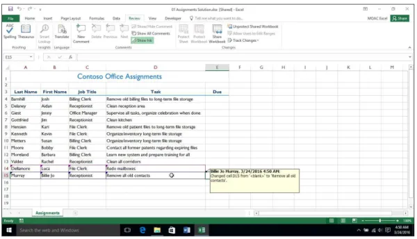
GET READY. LAUNCH Excel 2016 if it is not already open. 1. OPEN the 01 Assignments.xlsx workbook for this lesson. 2. SAVE the workbook as 01 Assignments Solution.xlsx.
3. Click the Review tab and then in the Changes group, click the Protect and Share Workbook button. The Protect Shared Workbook dialog box opens.
4. In the dialog box, click Sharing with track changes. When you choose this option, the Password text box becomes active. You can assign a password, but it is not necessary. Click OK.
5. Click OK when asked if you want to save the workbook and continue. You have now marked the workbook to track changes.
PAUSE. LEAVE the workbook open for the next exercise.
You can turn change tracking off by clicking the Unprotect Shared Workbook button, which was named Protect and Share Workbook before you completed the preceding exercise.
The Advanced tab of the Share Workbook dialog box allows you to customize the shared use of the workbook. These options are normally set by the workbook author before the workbook is shared. In this exercise, you modify these options.
STEP BY STEP Set Track Change Options
GET READY. USE the workbook from the previous exercise.
1. On the Review tab, in the Changes group, click Share Workbook. The Share Workbook dialog box opens.
3. In the Keep change history for box, click the scroll arrow to display 35.
4. Click the Automatically every option button so the file automatically saves every 15 minutes (the default for this setting).
5. Click OK to accept the default settings for the remainder of the options.
PAUSE. SAVE the workbook and LEAVE it open for the next exercise.
Take Note Turning off Track Changes removes the change history and removes the shared status of the work-book, but changes already shown in the document will remain until you accept or reject them.
Inserting Tracked Changes
When you open a shared workbook, Track Changes is automatically turned on. In most cases, the workbook owner has entered a password to prevent a user from turning off Track Changes. Thus, any text you type in the workbook is tracked.
STEP BY STEP Insert Tracked Changes
GET READY. USE the workbook from the previous exercise.
1. On the Review tab, in the Changes group, click Track Changes. In the drop-down list that appears, click Highlight Changes. The Highlight Changes dialog box opens. The Track changes while editing box is selected, but inactive because Track Changes was activated when you shared the workbook.
2. In the When drop-down box, click the down arrow and then click All. In the Who check box and drop-down list, check the box and then select Everyone. The dialog box should appear as shown in Figure 1-15.
Figure 1-14
Advanced tab in the Share Workbook dialog box
Figure 1-15
3. The Highlight changes on screen option is already selected. Click OK. If a warning box appears, click OK to accept.
4. Click the File tab and then click Options. The Excel Options dialog box opens.
5. In the General category, under Personalize your copy of Microsoft Office, in the User name box, type Luca Dellamore. Click OK. You have changed the document user name that will be listed in the Track Changes.
Take Note Make a note of the name that you remove. You will restore the original user name later in this lesson.
6. Click cell A14 and type the following information in each of the columns: Dellamore Luca File Clerk Redo mailboxes
7. As you enter these changes, a colored triangle and comment box appear for each entry made. This makes it easy to view the changes later.
8. On the Quick Access Toolbar, click Save to save the changes you made under the user name Luca Dellamore.
9. Click the File tab and then select Options.
10. In the User name box, type Billie Jo Murray. Click OK. You are once again changing the user name and applying it to the document.
11. Click cell A15 and type the following information in each of the columns: Murray Billie Jo Receptionist Remove all old contacts
12. Move the mouse pointer to cell D15. The person’s name who made the change, the date and time of the change, and the change itself appear in a ScreenTip as shown in Figure 1-16.
13. Look at the ScreenTips for the other cells in rows 14 and 15.
PAUSE. SAVE the workbook and LEAVE it open for the next exercise.
On a network, you do not see changes made by other users until both they and you save your changes. Note that when you work in a network environment, you can click Share Workbook in the Changes group and see a list of other users (on the Editing tab) who have the workbook open.
Sometimes conflicts occur when two users edit a shared workbook and try to save changes that affect the same cell. When the second user tries to save the workbook, Excel displays the Resolve Conflicts dialog box. Depending on the options established when the workbook was created and shared, you can either keep your change or accept the change made by the other user.
Figure 1-16
You can also display a list that shows how past conflicts have been resolved. These can be viewed on a separate worksheet that displays the name of the person who made the change, when and where it was made, what data was deleted or replaced, and how conflicts were resolved.
Deleting Your Changes
Changes become a part of the change history only when you save the workbook. If you change your mind before saving, you can edit or delete changes. Changes must be saved before you can accept or reject them. When you have saved your workbook and you want to delete a change, you can either enter new data or reject the change you made before saving.
STEP BY STEP Delete Your Changes
GET READY. USE the workbook from the previous exercise. 1. Click the File tab and then click Options.
2. In the General category, under Personalize your copy of Microsoft Office, in the User name box, type Erin Hagens. Click OK. You have again changed the user of the workbook for change tracking purposes.
3. Select cell A16 and type the following information in each of the columns: Hagens Erin Receptionist Clean all corridors
4. Click cell D11 and then edit the cell so patients is spelled correctly. Change patents to patients.
5. On the Review tab, click Track Changes and then from the drop-down menu that displays, click Accept/Reject Changes. Excel displays a message box confirming that you want to save the workbook. Click OK. The Select Changes to Accept or Reject dialog box opens.
6. In the Select Changes to Accept or Reject dialog box, click the Who drop-down arrow, select Erin Hagens, and then click OK. You have just asked Excel to return only the tracked changes made by Erin Hagens. Excel highlights row 16 with green dashes where Hagens’ information is typed in.
Take Note The order of the accept or reject changes may appear differently. Accept the change in D11 but reject all other changes.
7. Click Reject. All four entries are removed.
8. When cell D11 is selected for the correction of the spelling of patients, click Accept.
PAUSE. SAVE the workbook and LEAVE it open for the next exercise.
If you replace another user’s data and you want to restore the original data, you should reject your change. If you instead delete text you entered as a replacement for other text, you will leave the cell or range blank. Rejecting your change restores the entry that you replaced.
Accepting and Rejecting Changes from Other Users
STEP BY STEP Accept Changes from Another User
GET READY. USE the workbook from the previous exercise. 1. Click the File tab and then click Options.
2. In the General category, under Personalize your copy of Microsoft Office, in the User name box, type Jim Giest. Click OK.
3. Click Track Changes and then select Accept/Reject Changes from the drop-down list. 4. Not yet reviewed will be selected by default. In the Who box, select Luca Dellamore.
Click OK. The Accept or Reject Changes dialog box is displayed.
5. Click Accept to accept each of the changes Luca made. The Accept or Reject Changes dialog box closes when you have accepted all changes made by Luca Dellamore.
PAUSE. SAVE the workbook and LEAVE it open for the next exercise.
Take Note You can also click the Collapse Dialog button in the Where box on the Select Changes to Accept or Reject dialog box and then select the cells that contain changes. You can then accept or reject the changes in their entirety. In this exercise, some changes were highlighted by cell and others were highlighted by row, and you could accept or reject changes to the selected cell or range.
As the owner of the Assignments workbook, the office manager in the following exercise has the authority to accept or reject changes by all users. Rejecting changes, however, does not prohibit a user from changing the data again. When all users have made the necessary changes, the owner can remove users and unshare the workbook.
STEP BY STEP Reject Changes from Another User
GET READY. USE the workbook from the previous exercise. 1. Click Track Changes and then click Accept/Reject Changes.
2. On the right side of the Where box, click the Collapse Dialog button.
3. Select the data in row 15 and then click the Expand Dialog button. Click OK to close the Select Changes to Accept or Reject dialog box. The Accept or Reject Changes dialog box is displayed.
4. Click Reject All. A dialog box will open to ask you if you want to remove all changes and not review them. Click OK. The data is removed and row 15 is now blank. 5. SAVE the workbook as 01 Assignments Edited Solution.xlsx.
PAUSE. LEAVE the workbook open for the next exercise.
When you have the opportunity to work with a shared workbook that is saved on a network, you will likely encounter conflicts when you attempt to save a change that affects the same cell as an-other user’s changes. In the Resolve Conflicts dialog box, you can read the information about each change and the conflicting changes made by another user. The options set on the Advanced tab of the Share Workbook dialog box determine how conflicts are resolved.
Removing Shared Status from a Workbook
STEP BY STEP Remove Shared Status from a Workbook
GET READY. USE the workbook from the previous exercise.
1. On the Review tab, in the Changes group, click Track Changes and then click Highlight Changes.
2. In the When box, All is selected by default. This tells Excel to search through all tracked changes made to the worksheet.
3. Clear the Who and Where check boxes if they are selected.
4. Click the List changes on a new sheet check box. Click OK. A History sheet is added to the workbook (see Figure 1-17).
5. On the History worksheet, in the upper-left corner of the worksheet, adjacent to the first column and first row, click the Select All button. Click the Home tab and then in the Clipboard group, click the Copy button.
6. Press Ctrl+N to open a new workbook.
7. In the new workbook, on the Home tab, in the Clipboard group, click Paste.
8. SAVE the new workbook as 01 Assignments History Solution. CLOSE the workbook. 9. In the shared workbook, click the Review tab, click Unprotect Shared Workbook and
then click Share Workbook. The Share Workbook dialog box is displayed. On the Editing tab, make sure that Jim Giest (the last user name changed in the Excel Options dialog box) is the only user listed in the Who has this workbook open now list, as shown in Figure 1-18.
10. Clear the Allow changes by more than one user at the same time check box. Click OK to close the dialog box.
11. A dialog box opens to prompt you about removing the workbook from shared use. Click Yes to turn off the workbook’s shared status. The word Shared is removed from the title bar and the History worksheet is deleted.
12. Click the File tab and then click Options.
13. In the General category, in the User name box, type your name (or the original user name, before it was changed in this lesson). Click OK.
SAVE the workbook and CLOSE it. Figure 1-17
When shared status has been removed from a workbook, changes can be made like they are made in any workbook. You can, of course, turn change tracking on again, which will automatically share the workbook.
Knowledge Assessment
Multiple Choice
Select the best response for each of the following statements.
1. Which of the following is the file extension used for Excel Template files?
a. .xlsm
b. .xltx c. .xlsx
d. .xlam
2. Which of the following demonstrates the general format of a formula that references a cell in a different worksheet?
a. CellAddress!SheetName b. SheetName#CellAddress
c. CellAddress#SheetName d. SheetName!CellAddress
3. Which of the following statements best describes how to copy macros from one workbook to another?
a. Drag the module from one project to another in the Project Explorer window of the Visual Basic Editor.
b. Use the Record Macro button on the Developer tab.
c. Use the Add-Ins button on the Developer tab.
d. Open the Visual Basic Editor and type RUN COPYMACROS in the Project Explorer window.
4. Which of the following represents the syntax for a structured reference to a field in an Excel table?
a. FieldName[TableName] b. TableName[FieldName]
c. [FieldName]TableName d. [TableName]FieldName Figure 1-18
5. Your co-worker sent you a workbook to update. You have entered new numbers in your worksheet, but the totals are not updating. Which of the following statements best describes how to remedy the problem?
a. Click the Share Workbook button on the Review tab.
b. Go to the cells with the totals that are not updating, press the F2 key and then press Enter to re-enter the formulas.
c. Click the Calculation Options button on the Formulas tab and change the calculation setting from Manual to Automatic.
d. Send the workbook back to your co-worker and have them fix it.
6. Which of the following methods is used to display a hidden tab on the ribbon?
a. On the View tab, in the Show group, click the Tabs button and select the tab you want to display.
b. Right-click any tab on the ribbon and select Display Hidden Tabs.
c. On the Home tab, in the Cells group, click Insert and then select Show Hidden Tabs.
d. Display the Excel Options dialog box, select Customize Ribbon, and then select the check box next to the name of the tab you want to add.
7. Which of the following statements best describes how to create a custom template of your own?
a. Click the File tab, select Save As, click Browse, and change the file type to .xltx.
b. Click the File tab, select Save As, click Browse, and change the file type to .xlsm.
c. Click the File tab, select Save As, click Browse, and change the file type to .xlam.
d. Click the File tab, select Options, click Save, select the Save as Template check box, and save the file as usual.
8. What is the name of the feature that saves copies of your files at specified intervals?
a. Protect Sheet
b. Track Changes
c. AutoRecover
d. Document Recovery
9. Which of the following would be considered a strong password based on the definition in this lesson?
a. Tsj1961x
b. 927%851*
c. 4Nw9!tP@
d. 239OAK$T
10. What is the name of the separate worksheet that temporarily lists all tracked changes in a shared workbook?
a. Changes
b. History
c. Review
d. Tracking
Projects
Project 1-1:
Customizing and Protecting an Excel TemplateIn this project, you will download and customize an Excel business expense report template. After unlocking the cells you want others to be able to edit, you will protect the worksheet and assign a password.
GET READY. LAUNCH Excel 2016 if it is not already open.
1. If you just opened Excel, you’re looking at the list of featured templates. If you do not see the list of featured templates, click the File tab and then click New.
3. Select the range C4:C7, and then on the Home tab, in the Cells group, click Format and select Lock Cell to deselect the option.
4. Repeat step 3 for the following cell ranges: F4:F7, J4:J8, M4:M8 and B14:M24.
5. Click the Review tab, and then in the Changes group, click Protect Sheet. The Protect Sheet dialog box opens.
6. In the Allow all users of this worksheet to list, ensure that the first two items are selected and then select the Format cells check box.
7. In the Password to unprotect sheet box, type P1&ex1! and then click OK. Enter the same password in the Reenter password to proceed box and then click OK. 8. Try to edit the text in cell B4. Excel displays an error message because this cell is
protected. Click OK to dismiss the message.
9. Edit the year in cells J5, J6, B14 and B15 to reflect the current year. Notice that you are able to edit these cells because you unlocked them before protecting the worksheet. 10. Click the Page Layout tab, click the Themes button, and select Damask. Excel won’t
allow you to change the design theme. Although you selected the option to allow users to format cells in step 6, this affects only the unlocked cells. Click OK to dismiss the message.
11. Click the Review tab and then click Unprotect Sheet. The Unprotect Sheet dialog box opens.
12. Type P1&ex1! in the Password box and then click OK.
13. Click the Page Layout tab, click the Themes button, and select Damask. Because the worksheet is unprotected, you are able to change the design theme.
14. Click the Review tab and then click Protect Sheet. The Protect Sheet dialog box opens. Type P1&ex1! in the Password box and then click OK. Enter the same password in the Reenter password to proceed box and then click OK.
15. Apply Bold and the Dark Blue font color to cell A1. Select the range B13:M13 and apply the Dark Blue, Text 2 fill color.
16. Press Ctrl+Home to return to the top of the worksheet. Your customized template should resemble Figure 1-19.
17. SAVE the workbook in the Excel Template (*.xltx) format as 01 Template Solution.xltx (change to another folder, if necessary) and then CLOSE it.
PAUSE. LEAVE Excel open to use in the next project. Figure 1-19
Project 1-2:
Copying a Macro between WorkbooksIn this project, you will copy an existing macro in a tour revenues workbook to a new workbook so that it can be reused in that workbook at a later date.
GET READY. LAUNCH Excel 2016 if it is not already open.
1. OPEN the 01 Revenues.xlsm workbook file for this exercise. If you see a Security Warning bar, click Enable Content to continue. Ensure that no other workbooks are open.
2. Press Ctrl+N to create a new workbook. SAVE the workbook in Excel Macro-Enabled Workbook (*.xlsm) format as 01 Revenues Solution.xlsm.
3. Display the Developer tab in the ribbon, if it isn’t already displayed. Click the Developer tab and then in the Code group, click the Visual Basic button.
4. Notice the Project Explorer window in the VBE. The window’s title begins with Project. If this is not visible, press Ctrl+R.
5. If necessary, widen the Project Explorer window a bit so that you can see enough of the workbook names to tell which one ends in Solution.
6. Click the [+] expand button to expand the branches in the 01 Revenues.xlsm workbook and the 01 Revenues Solution.xlsm workbook, as necessary.
7. In the tree structure for the 01 Revenues.xlsm workbook, you will see a branch labeled Modules. Under that branch you will see a module named Module1. Double-click Module1 to see the associated macro in the Code window. Notice that the name of the macro is CustomSubtotals.
8. In the Project Explorer window, click the Module1 module in the 01 Revenues.xlsm tree, drag it inside the tree structure for the 01 Revenues Solution.xlsm workbook and then release the mouse button.
9. The tree structure under the 01 Revenues Solution.xlsm workbook will now have a Modules folder. Click the [+] expand button to expand the folder (see Figure 1-20).
10. In the VBE window, click File and then click Close and Return to Microsoft Excel. Display the new 01 Revenues Solution.xlsm workbook, if necessary.
11. On the Developer tab, in the Code group, click the Macros button. In the Macro dialog box, change the Macros in value to This Workbook. Notice that the CustomSubtotals macro now appears in the new workbook. Click Cancel to close the Macro dialog box. 12. SAVE the 01 Revenues Solution.xlsm workbook and CLOSE it. Then, CLOSE the 01
Revenues.xlsm workbook without saving changes. EXIT Excel.
Figure 1-20
Applying Custom Formatting
and Layouts
2
27
LESSON SKILL MATRIX
Skills Exam Objective Objective Number
Applying Custom Formats and Validating Data
Create custom number formats.
Populate cells by using advanced Fill Series options. Configure data validation.
2.1.1 2.1.2 2.1.3
Applying Conditional Formatting and Filtering
Create custom conditional formatting rules.
Create conditional formatting rules that use formulas. Manage conditional formatting rules.
2.2.1 2.2.2 2.2.3
Creating Custom Workbook Elements
Create and modify custom themes. Create custom color formats.
Manage multiple options for +Body and +Heading fonts. Create and modify cell styles.
Create and modify simple macros. Insert and configure form controls.
2.3.3 2.3.1 2.4.3 2.3.2 2.3.4 2.3.5
Preparing a Workbook for Internationalization
Display data in multiple international formats. Apply international currency formats.
2.4.1 2.4.2
APPLYING CUSTOM FORMATS AND VALIDATING DATA
Although you can apply common number formats from the ribbon, you may occasionally want to create a custom number format to fit your needs. Custom formats can be specified using the Cus-tom category on the Number tab of the Format Cells dialog box. Excel also provides options that allow you to populate cells using advanced Fill Series options that include linear and growth series.
When typing new data in a workbook from a paper source—especially several records at once— it’s easy for anyone to type the wrong digits or characters, especially in a field where a single char-acter denotes a type, such as a senior citizen or a child, or such as a dog or a cat. Data validation helps to ensure that data gets entered correctly, before it gets processed incorrectly.
Applying Custom Number Formats
In Excel, the same number can appear differently in a cell depending on its number format. For example, 0.25, 1/4, and 6:00 A.M. are all the exact same number in Excel. Changing the number format has the same impact on the cell’s value as changing its color—none. In this section, we will look at some of the other things you can do with number formatting.
You can use formatting controls on the ribbon to quickly change your cells’ number formats to the most commonly used formats. Now we’re going to explore custom number formats. The first thing to understand when defining custom number formats is that Excel allows four number formats in every cell, and they are separated with semicolons. The basic structure is:
<Format for Positive Numbers> ; <Negative Numbers> ; <Zeroes> ; <Text>
Code Description
0 (zero) Digit placeholder. This means the number always displays, even if it’s not significant. A format of 000.00 would display the number 3.3 as 003.30
# Digit placeholder; doesn’t show insignificant zeroes. The # symbol comes into play mostly when placing your thousands separators. A format of #,##0.## would display the number 3.3 as 3.3
? The question mark is also a digit placeholder. It follows rules that are similar to the # placeholder described above—if there’s a non-zero number it will display the number, but it won’t display a zero. However, unlike the # symbol, for a zero the ? will display a space, not nothing. This means that if you use a format like 0.0?? Excel would align the numbers’ decimals vertically, three digit-spaces from the right. The question mark also gets a lot of use when formatting fractions.
. The period displays the decimal point in a number.
, The thousands separator. About the only time the decimal point (.) and thousands separator (,) can get “interesting” is if you are working with interna-tional workbooks and you have modified the advanced options by deselecting the Use system separators check box. If you do that, then Excel will update any custom formats to use whichever separators you’ve indicated in your advanced options.
% Displays the number as a percent—multiplies the number by 100 and places a % symbol after it. Note that the value doesn’t change; 99% still has a value of 0.99. When typing numbers manually, Excel interprets anything between 1 and 100 to be a shorthand percent. In other words, even though 99 would really be 9900%, if a cell is formatted as 0.00% and you type 99, you’ll get 99%, which is 0.99. If you type 0.99 you’ll also get 99%, which is 0.99. If you need a real 99, then you’ll need to type 9900. If you need 0.99%, you’ll need to type 0.0099.
/ The fraction indicator. Use this in conjunction with the question mark (?) character. The ? will limit the number of digits Excel uses in the numerator or denominator.
E+ or E− Scientific Notation. If you put a “+1” after the E then you’ll always see a sign for the exponent. If you put a “−” then you’ll only see a sign for negative exponents. Note that while you can type a number in scientific notation by using a lower-case “e”, you cannot use a lowerlower-case “e” in the number format specification. Excel always displays scientific notation using an uppercase “E”.
$ € ¥ £ + − ( ) space /
These symbols along with : ^ ’ { }, < >= ! ~ can be specified in a number format without enclosing the character inside double quotation marks.
\ Backslash is the literal demarcation character. This means that whatever comes directly after the backslash gets shown.
_ Underscore. This is a special formatting character because, like the backslash, it tells Excel to do something special based on whatever character comes next. In the case of the underscore, it means “insert space equal to this character’s width.” The most common use is _) at the end of a positive number format, where the negative numbers are enclosed in parentheses. By adding the width of the closing parenthesis, all the decimal points in the column remain aligned.
* The asterisk means “repeat after me.” Excel will apply all of the formatting and if there is any space left in the cell, it will then use whatever character follows the asterisk to fill out the rest of the cell. The * is used most frequently in conjunc-tion with a space in the Accounting number formats. The Accounting formats begin with a $ followed by “*” (without the double quotes) which tells Excel to fill any unused width with spaces after the $.
Code Description
@ The at (@) symbol is the text placeholder.
d or dd Days as digits. If you use one d, you’ll get 0 – 31. If you use two d’s, you’ll get 00 – 31.
ddd or dddd Days as day of the week name. If you use three d’s, you’ll get Sun – Sat. If you use four d’s, you’ll get Sunday – Saturday. There is no cell number format that displays the day of the week as a number, for example, displaying a 1 for a Sunday. You would need to use the WEEKDAY function for that purpose.
m or mm Months as digits. If you use one m, you’ll get 0 – 12. If you use two m’s, you’ll get 00 – 12.
mmm or mmmm Name of the month. Three m’s displays Jan – Dec. Four m’s displays January – December.
mmmmm This one is counter-intuitive. Because the single m format gives you a digit, in order to get a one-letter month you use five m’s, so you get J – D. This number format is most useful on charts where you might use a number format of mmmmm to show J F M A M J . . . across the x-axis of a chart.
yy or yyyy Year as 00 – 99 or 1900 – 9999.
h or hh Hours as 0 – 24 or 00 – 24. <