• • The buck stops here — get straightforward guidance on how to
put information into Excel workbooks so that you can begin to analyze it
• You oughta know — find must-know, useful tidbits about statistics, analyzing data, and visually presenting data that will make sense of the stuff you’re digging for
• Behold the power — discover the most powerful data analysis tools that Excel provides, its cross-tabulation capabilities PivotTable and PivotChart
• You’re analyzing data, darling — get to know the more sophisticated tools provided by Excel data analysis add-ons, like t-test, z-test, scatter plot, regression, ANOVA, and Fourier
Exc
Author of
QuickBooks For Dummies®
E. C. Nelson
Learn to:
•
Navigate and analyze data
•
Work with external databases,
PivotTables, and PivotCharts
•
Use Excel for statistical and financial
functions
•
Make the most of the latest features
of Excel 2013
Excel
®
Data Analysis
2nd Edition
Making Everything E
asier!
™Start with
FREE
Cheat Sheets
Cheat Sheets include
• Checklists
• Charts
• Common Instructions
• And Other Good Stuff!
Get Smart at Dummies.com
Dummies.com makes your life easier with 1,000s
of answers on everything from removing wallpaper
to using the latest version of Windows.
Check out our
• Videos
• Illustrated Articles
• Step-by-Step Instructions
Plus, each month you can win valuable prizes by entering
our Dummies.com sweepstakes. *
Want a weekly dose of Dummies? Sign up for Newsletters on
• Digital Photography
• Microsoft Windows & Office
• Personal Finance & Investing
• Health & Wellness
• Computing, iPods & Cell Phones
• eBay
• Internet
• Food, Home & Garden
Find out “HOW” at Dummies.com
Get More and Do More at Dummies.com
®
To access the Cheat Sheet created specifically for this book, go to
Excel
®
Data
Analysis
2nd Edition
Excel® Data Analysis For Dummies,® 2nd Edition
Published by: John Wiley & Sons, Inc., 111 River Street, Hoboken, NJ 07030-5774, www.wiley.com
Copyright © 2014 by John Wiley & Sons, Inc., Hoboken, New Jersey Published simultaneously in Canada
No part of this publication may be reproduced, stored in a retrieval system or transmitted in any form or by any means, electronic, mechanical, photocopying, recording, scanning or otherwise, except as permitted under Sections 107 or 108 of the 1976 United States Copyright Act, without the prior written permission of the Publisher. Requests to the Publisher for permission should be addressed to the Permissions Department, John Wiley & Sons, Inc., 111 River Street, Hoboken, NJ 07030, (201) 748-6011, fax (201) 748-6008, or online at
http://www.wiley.com/go/permissions.
Trademarks: Wiley, For Dummies, the Dummies Man logo, Dummies.com, Making Everything Easier, and related trade dress are trademarks or registered trademarks of John Wiley & Sons, Inc. and may not be used without written permission. Excel is a registered trademark of Microsoft Corporation. All other trademarks are the property of their respective owners. John Wiley & Sons, Inc. is not associated with any product or vendor mentioned in this book.
LIMIT OF LIABILITY/DISCLAIMER OF WARRANTY: THE PUBLISHER AND THE AUTHOR MAKE NO REPRESENTATIONS OR WARRANTIES WITH RESPECT TO THE ACCURACY OR COMPLETENESS OF THE CONTENTS OF THIS WORK AND SPECIFICALLY DISCLAIM ALL WARRANTIES, INCLUDING WITHOUT LIMITATION WARRANTIES OF FITNESS FOR A PARTICULAR PURPOSE. NO WARRANTY MAY BE CREATED OR EXTENDED BY SALES OR PROMOTIONAL MATERIALS. THE ADVICE AND STRATEGIES CONTAINED HEREIN MAY NOT BE SUITABLE FOR EVERY SITUATION. THIS WORK IS SOLD WITH THE UNDERSTANDING THAT THE PUBLISHER IS NOT ENGAGED IN RENDERING LEGAL, ACCOUNTING, OR OTHER PROFESSIONAL SERVICES. IF PROFESSIONAL ASSISTANCE IS REQUIRED, THE SERVICES OF A COMPETENT PROFESSIONAL PERSON SHOULD BE SOUGHT. NEITHER THE PUBLISHER NOR THE AUTHOR SHALL BE LIABLE FOR DAMAGES ARISING HEREFROM. THE FACT THAT AN ORGANIZATION OR WEBSITE IS REFERRED TO IN THIS WORK AS A CITATION AND/OR A POTENTIAL SOURCE OF FURTHER INFORMATION DOES NOT MEAN THAT THE AUTHOR OR THE PUBLISHER ENDORSES THE INFORMATION THE ORGANIZATION OR WEBSITE MAY PROVIDE OR RECOMMENDATIONS IT MAY MAKE. FURTHER, READERS SHOULD BE AWARE THAT INTERNET WEBSITES LISTED IN THIS WORK MAY HAVE CHANGED OR DISAPPEARED BETWEEN WHEN THIS WORK WAS WRITTEN AND WHEN IT IS READ.
For general information on our other products and services, please contact our Customer Care Department within the U.S. at 877-762-2974, outside the U.S. at 317-572-3993, or fax 317-572-4002. For technical support, please visit www.wiley.com/techsupport.
Wiley publishes in a variety of print and electronic formats and by print-on-demand. Some material included with standard print versions of this book may not be included in e-books or in print-on-demand. If this book refers to media such as a CD or DVD that is not included in the version you purchased, you may download this material at http://booksupport.wiley.com. For more information about Wiley prod-ucts, visit www.wiley.com.
Library of Congress Control Number: 2013957980
ISBN 978-1-118-89809-3 (pbk); ISBN 978-1-118-89808-6 (ebk); ISBN 978-1-118-89810-9 (ebk)
Contents at a Glance
Introduction ... 1
Part I: Where’s the Beef? ... 7
Chapter 1: Introducing Excel Tables ... 9
Chapter 2: Grabbing Data from External Sources ... 31
Chapter 3: Scrub-a-Dub-Dub: Cleaning Data ... 57
Part II: PivotTables and PivotCharts ... 79
Chapter 4: Working with PivotTables ... 81
Chapter 5: Building PivotTable Formulas ... 107
Chapter 6: Working with PivotCharts ... 127
Chapter 7: Customizing PivotCharts ... 141
Part III: Advanced Tools ... 155
Chapter 8: Using the Database Functions ... 157
Chapter 9: Using the Statistics Functions ... 177
Chapter 10: Descriptive Statistics... 225
Chapter 11: Inferential Statistics ... 245
Chapter 12: Optimization Modeling with Solver ... 263
Part IV: The Part of Tens ... 287
Chapter 13: Ten Things You Ought to Know about Statistics ... 289
Chapter 14: Almost Ten Tips for Presenting Table Results and Analyzing Data ... 301
Chapter 15: Ten Tips for Visually Analyzing and Presenting Data ... 307
Appendix: Glossary of Data Analysis
and Excel Terms ... 319
Table of Contents
Introduction ... 1
About This Book ... 1
What You Can Safely Ignore ... 1
What You Shouldn’t Ignore (Unless You’re a Masochist) ... 2
Foolish Assumptions ... 3
How This Book Is Organized ... 3
Part I: Where’s the Beef? ... 3
Part II: PivotTables and PivotCharts ... 3
Part III: Advanced Tools ... 3
Part IV: The Part of Tens ... 4
Icons Used in This Book ... 4
Beyond the Book ... 5
Where to Go from Here ... 5
Part I: Where’s the Beef? ... 7
Chapter 1: Introducing Excel Tables . . . . 9
What Is a Table and Why Do I Care? ... 9
Building Tables ... 12
Exporting from a database ... 12
Building a table the hard way... 12
Building a table the semi-hard way ... 12
Analyzing Table Information ... 16
Simple statistics ... 16
Sorting table records ... 18
Using AutoFilter on a table ... 21
Undoing a filter ... 23
Turning off filter ... 23
Using the custom AutoFilter ... 23
Filtering a filtered table ... 25
Using advanced filtering ... 26
Chapter 2: Grabbing Data from External Sources . . . . 31
Getting Data the Export-Import Way ... 31
Exporting: The first step ... 32
Importing: The second step (if necessary) ... 37
Querying External Databases and Web Page Tables ... 44
Running a web query ... 45
Importing a database table ... 47
Querying an external database ... 49
Excel Data Analysis For Dummies, 2nd Edition
vi
Chapter 3: Scrub-a-Dub-Dub: Cleaning Data . . . . 57
Editing Your Imported Workbook ... 57
Delete unnecessary columns ... 58
Delete unnecessary rows ... 58
Resize columns... 58
Resize rows ... 60
Erase unneeded cell contents ... 61
Format numeric values ... 61
Copying worksheet data ... 62
Moving worksheet data ... 62
Replacing data in fields ... 62
Cleaning Data with Text Functions ... 63
What’s the big deal, Steve? ... 63
The answer to some of your problems ... 64
The CLEAN function ... 65
The CONCATENATE function ... 65
The EXACT function ... 66
The FIND function ... 67
The FIXED function ... 67
The LEFT function... 68
The LEN function ... 68
The LOWER function ... 68
The MID function ... 69
The PROPER function ... 69
The REPLACE function ... 70
The REPT function ... 70
The RIGHT function ... 70
The SEARCH function ... 71
The SUBSTITUTE function ... 71
The T function ... 72
The TEXT function ... 72
The TRIM function ... 73
The UPPER function ... 73
The VALUE function ... 73
Converting text function formulas to text ... 74
Using Validation to Keep Data Clean ... 74
Part II: PivotTables and PivotCharts ... 79
Chapter 4: Working with PivotTables . . . . 81
Looking at Data from Many Angles ... 81
Getting Ready to Pivot ... 82
vii
Table of Contents
Pivoting and re-pivoting ... 88
Filtering pivot table data ... 89
Refreshing pivot table data ... 91
Sorting pivot table data ... 92
Pseudo-sorting ... 94
Grouping and ungrouping data items ... 94
Selecting this, selecting that ... 96
Where did that cell’s number come from? ... 96
Setting value field settings ... 97
Customizing How Pivot Tables Work and Look ... 99
Setting pivot table options ... 99
Formatting pivot table information ... 103
Chapter 5: Building PivotTable Formulas . . . . 107
Adding Another Standard Calculation ... 107
Creating Custom Calculations ... 111
Using Calculated Fields and Items ... 115
Adding a calculated field... 115
Adding a calculated item ... 117
Removing calculated fields and items ... 120
Reviewing calculated field and calculated item formulas ... 121
Reviewing and changing solve order ... 122
Retrieving Data from a Pivot Table ... 123
Getting all the values in a pivot table ... 123
Getting a value from a pivot table ... 124
Arguments of the GETPIVOTDATA function ... 126
Chapter 6: Working with PivotCharts . . . . 127
Why Use a Pivot Chart? ... 127
Getting Ready to Pivot ... 128
Running the PivotTable Wizard ... 129
Fooling Around with Your Pivot Chart ... 133
Pivoting and re-pivoting ... 134
Filtering pivot chart data ... 134
Refreshing pivot chart data ... 137
Grouping and ungrouping data items ... 138
Using Chart Commands to Create Pivot Charts ... 139
Chapter 7: Customizing PivotCharts . . . . 141
Selecting a Chart Type ... 141
Working with Chart Styles ... 142
Changing Chart Layout ... 143
Chart and axis titles ... 143
Chart legend ... 145
Excel Data Analysis For Dummies, 2nd Edition
viii
Chart data tables ... 147
Chart axes ... 149
Chart gridlines ... 150
Changing a Chart’s Location ... 150
Formatting the Plot Area ... 152
Formatting the Chart Area ... 152
Chart fill patterns ... 153
Chart area fonts ... 153
Formatting 3-D Charts ... 154
Formatting the walls of a 3-D chart... 154
Using the 3-D View command ... 154
Part III: Advanced Tools ... 155
Chapter 8: Using the Database Functions . . . . 157
Quickly Reviewing Functions ... 157
Understanding function syntax rules ... 158
Entering a function manually ... 158
Entering a function with the Function command ... 159
Using the DAVERAGE Function ... 163
Using the DCOUNT and DCOUNTA Functions ... 166
Using the DGET Function ... 168
Using the DMAX and DMAX Functions ... 169
Using the DPRODUCT Function ... 170
Using the DSTDEV and DSTDEVP Functions ... 171
Using the DSUM Function ... 173
Using the DVAR and DVARP Functions ... 174
Chapter 9: Using the Statistics Functions . . . . 177
Counting Items in a Data Set ... 177
COUNT: Counting cells with values ... 178
COUNTA: Alternative counting cells with values ... 179
COUNTBLANK: Counting empty cells ... 179
COUNTIF: Counting cells that match criteria ... 179
PERMUT: Counting permutations ... 180
COMBIN: Counting combinations ... 180
Means, Modes, and Medians ... 181
AVEDEV: An average absolute deviation ... 181
AVERAGE: Average ... 182
AVERAGEA: An alternate average ... 182
TRIMMEAN: Trimming to a mean ... 183
MEDIAN: Median value ... 183
ix
Table of Contents
Finding Values, Ranks, and Percentiles ... 185
MAX: Maximum value ... 185
MAXA: Alternate maximum value ... 185
MIN: Minimum value ... 185
MINA: Alternate minimum value ... 186
LARGE: Finding the kth largest value ... 186
SMALL: Finding the kth smallest value ... 186
RANK: Ranking an array value... 187
PERCENTRANK: Finding a percentile ranking ... 188
PERCENTILE: Finding a percentile ranking ... 189
FREQUENCY: Frequency of values in a range ... 189
PROB: Probability of values... 190
Standard Deviations and Variances ... 192
STDEV: Standard deviation of a sample ... 193
STDEVA: Alternate standard deviation of a sample ... 193
STDEVP: Standard deviation of a population ... 194
STDEVPA: Alternate standard deviation of a population ... 194
VAR: Variance of a sample ... 194
VARA: Alternate variance of a sample ... 195
VARP: Variance of a population ... 195
VARPA: Alternate variance of a population ... 196
COVARIANCE.P and COVARIANCE.S: Covariances ... 196
DEVSQ: Sum of the squared deviations ... 196
Normal Distributions ... 197
NORM.DIST: Probability X falls at or below a given value ... 197
NORM.INV: X that gives specified probability ... 198
NORM.S.DIST: Probability variable within z-standard deviations ... 198
NORM.S.INV: z-value equivalent to a probability ... 199
STANDARDIZE: z-value for a specified value ... 199
CONFIDENCE: Confidence interval for a population mean ... 200
KURT: Kurtosis ... 201
SKEW and SKEW.P: Skewness of a distribution ... 201
t-distributions ... 202
T.DIST: Left-tail Student t-distribution ... 202
T.DIST.RT: Right-tail Student t-distribution ... 203
T.DIST.2T: Two-tail Student t-distribution ... 203
T.INV: Left-tailed Inverse of Student t-distribution ... 204
T.INV.2T: Two-tailed Inverse of Student t-distribution ... 204
T.TEST: Probability two samples from same population ... 204
f-distributions ... 205
F.DIST: Left-tailed f-distribution probability ... 205
F.DIST.RT: Right-tailed f-distribution probability ... 206
F.INV:Left-tailed f-value given f-distribution probability... 206
F.INV.RT:Right-tailed f-value given f-distribution probability ... 207
Excel Data Analysis For Dummies, 2nd Edition
x
Binomial Distributions ... 207
BINOM.DIST: Binomial probability distribution ... 208
BINOM.INV: Binomial probability distribution ... 208
BINOM.DIST.RANGE: Binomial probability of Trial Result ... 209
NEGBINOM.DIST: Negative binominal distribution ... 210
CRITBINOM: Cumulative binomial distribution ... 210
HYPGEOM.DIST: Hypergeometric distribution ... 211
Chi-Square Distributions ... 211
CHISQ.DIST.RT: Chi-square distribution ... 212
CHISQ.DIST: Chi-square distribution ... 213
CHISQ.INV.RT: Right-tailed chi-square distribution probability ... 213
CHISQ.INV: Left-tailed chi-square distribution probability ... 214
CHISQ.TEST: Chi-square test ... 214
Regression Analysis ... 215
FORECAST: Forecast dependent variables using a best-fit line ... 215
INTERCEPT: y-axis intercept of a line... 216
LINEST ... 216
SLOPE: Slope of a regression line ... 216
STEYX: Standard error ... 217
TREND ... 217
LOGEST: Exponential regression ... 217
GROWTH: Exponential growth ... 217
Correlation ... 218
CORREL: Correlation coefficient ... 218
PEARSON: Pearson correlation coefficient ... 218
RSQ: r-squared value for a Pearson correlation coefficient ... 218
FISHER ... 219
FISHERINV ... 219
Some Really Esoteric Probability Distributions ... 219
BETA.DIST: Cumulative beta probability density ... 219
BETA.INV: Inverse cumulative beta probability density ... 220
EXPON.DIST: Exponential probability distribution ... 220
GAMMA.DIST: Gamma distribution probability ... 221
GAMMAINV: X for a given gamma distribution probability ... 222
GAMMALN: Natural logarithm of a gamma distribution ... 222
LOGNORMDIST: Probability of lognormal distribution ... 222
LOGINV: Value associated with lognormal distribution probability ... 222
POISSON: Poisson distribution probabilities ... 223
WEIBULL: Weibull distribution ... 223
ZTEST: Probability of a z-test ... 224
Chapter 10: Descriptive Statistics . . . . 225
xi
Table of Contents
Exponential Smoothing ... 237
Generating Random Numbers ... 239
Sampling Data ... 241
Chapter 11: Inferential Statistics . . . . 245
Using the t-test Data Analysis Tool ... 246
Performing z-test Calculations ... 249
Creating a Scatter Plot ... 251
Using the Regression Data Analysis Tool ... 254
Using the Correlation Analysis Tool ... 257
Using the Covariance Analysis Tool ... 258
Using the ANOVA Data Analysis Tools ... 260
Creating an f-test Analysis ... 261
Using Fourier Analysis ... 262
Chapter 12: Optimization Modeling with Solver . . . . 263
Understanding Optimization Modeling ... 263
Optimizing your imaginary profits ... 264
Recognizing constraints ... 264
Setting Up a Solver Worksheet ... 265
Solving an Optimization Modeling Problem ... 268
Reviewing the Solver Reports ... 273
The Answer Report ... 273
The Sensitivity Report ... 275
The Limits Report ... 276
Some other notes about Solver reports ... 277
Working with the Solver Options ... 277
Using the All Methods options ... 278
Using the GRG Nonlinear tab ... 279
Using the Evolutionary tab ... 281
Saving and reusing model information ... 282
Understanding the Solver Error Messages ... 282
Solver has found a solution ... 283
Solver has converged to the current solution ... 283
Solver cannot improve the current solution ... 283
Stop chosen when maximum time limit was reached ... 283
Solver stopped at user’s request ... 284
Stop chosen when maximum iteration limit was reached... 284
Objective Cell values do not converge... 284
Solver could not find a feasible solution ... 284
Linearity conditions required by this LP Solver are not satisfied ... 285
The problem is too large for Solver to handle ... 285
Solver encountered an error value in a target or constraint cell ... 285
There is not enough memory available to solve the problem ... 286
Excel Data Analysis For Dummies, 2nd Edition
xii
Part IV: The Part of Tens ... 287
Chapter 13: Ten Things You Ought to Know about Statistics . . . . 289
Descriptive Statistics Are Straightforward ... 290
Averages Aren’t So Simple Sometimes ... 290
Standard Deviations Describe Dispersion ... 291
An Observation Is an Observation ... 292
A Sample Is a Subset of Values ... 293
Inferential Statistics Are Cool but Complicated ... 293
Probability Distribution Functions Aren’t Always Confusing ... 294
Uniform distribution ... 294
Normal distribution ... 295
Parameters Aren’t So Complicated ... 296
Skewness and Kurtosis Describe a Probability Distribution’s Shape ... 297
Confidence Intervals Seem Complicated at First, but Are Useful ... 297
Chapter 14: Almost Ten Tips for Presenting Table Results and
Analyzing Data . . . . 301
Work Hard to Import Data ... 301
Design Information Systems to Produce Rich Data ... 302
Don’t Forget about Third-Party Sources ... 303
Just Add It ... 303
Always Explore Descriptive Statistics ... 304
Watch for Trends ... 304
Slicing and Dicing: Cross-Tabulation ... 305
Chart It, Baby ... 305
Be Aware of Inferential Statistics ... 305
Chapter 15: Ten Tips for Visually Analyzing and
Presenting Data . . . . 307
Using the Right Chart Type ... 307
Using Your Chart Message as the Chart Title ... 309
Beware of Pie Charts ... 310
Consider Using Pivot Charts for Small Data Sets ... 310
Avoiding 3-D Charts ... 312
Never Use 3-D Pie Charts ... 313
Be Aware of the Phantom Data Markers ... 314
Use Logarithmic Scaling ... 315
Don’t Forget to Experiment ... 317
Get Tufte ... 317
Introduction
S
o here’s a funny deal: You know how to use Excel. You know how to create simple workbooks and how to print stuff. And you can even, with just a little bit of fiddling, create cool-looking charts.But I bet that you sometimes wish that you could do more with Excel. You sometimes wish, I wager, that you could use Excel to really gain insights into the information, the data, that you work with in your job.
Using Excel for data analysis is what this book is all about. This book assumes that you want to use Excel to learn new stuff, discover new secrets, and gain new insights into the information that you’re already working with in Excel — or the information stored electronically in some other format, such as in your accounting system or from your web server’s analytics.
About This Book
This book isn’t meant to be read cover to cover like a Dan Brown page-turner. Rather, it’s organized into tiny, no-sweat descriptions of how to do the things that must be done. Hop around and read the chapters that interest you.
If you’re the sort of person who, perhaps because of a compulsive bent, needs to read a book cover to cover, that’s fine. I recommend that you delve in to the chapters on inferential statistics, however, only if you’ve taken at least a couple of college-level statistics classes. But that caveat aside, feel free. After all, maybe Dancing with the Stars is a rerun tonight.
What You Can Safely Ignore
This book provides a lot of information. That’s the nature of a how-to refer-ence. So I want to tell you that it’s pretty darn safe for you to blow off some chunks of the book.
2
Excel Data Analysis For Dummies, 2nd Edition
bold-faced description of what the step entails. Underneath that bold-faced step description, I provide detailed information about what happens after you perform that action. Sometimes I also offer help with the mechanics of the step, like this:
1. Press Enter.
Find the key that’s labeled Enter. Extend your index finger so that it rests ever so gently on the Enter key. Then, in one sure, fluid motion, press the key by using your index finger. Then release the key.
Okay, that’s kind of an extreme example. I never actually go into that much detail. My editor won’t let me. But you get the idea. If you know how to press Enter, you can just do that and not read further. If you need help — say with the finger-depression part or the finding-the-right-key part — you can read the nitty-gritty details.
You can also skip the paragraphs flagged with the Technical Stuff icon. These icons flag information that’s sort of tangential, sort of esoteric, or sort of questionable in value . . . at least for the average reader. If you’re really inter-ested in digging into the meat of the subject being discussed, go ahead and read ’em. If you’re really just trying to get through your work so that you can get home and watch TV with your kids, skip ’em.
I might as well also say that you don’t have to read the information provided in the paragraphs marked with a Tip icon, either. I assume that you want to know an easier way to do something. But if you like to do things the hard way because that improves your character and makes you tougher, go ahead and skip the Tip icons.
What You Shouldn’t Ignore (Unless
You’re a Masochist)
By the way, don’t skip the Warning icons. They’re the text flagged with a picture of a 19th century bomb. They describe some things that you really shouldn’t do.
Out of respect for you, I don’t put stuff in these paragraphs such as, “Don’t smoke.” I figure that you’re an adult. You get to make your own lifestyle decisions.
3
Introduction
Foolish Assumptions
I assume just three things about you:
✓ You have a PC with a recent version of Microsoft Excel 2007 installed.
✓ You know the basics of working with your PC and Microsoft Windows.
✓ You know the basics of working with Excel, including how to start and stop Excel, how to save and open Excel workbooks, and how to enter text and values and formulas into worksheet cells.
How This Book Is Organized
This book is organized into five parts:
Part I: Where’s the Beef?
In Part I, I discuss how you get data into Excel workbooks so that you can begin to analyze it. This is important stuff, but fortunately most of it is pretty straightforward. If you’re new to data analysis and not all that fluent yet in working with Excel, you definitely want to begin in Part I.
Part II: PivotTables and PivotCharts
In the second part of this book, I cover what are perhaps the most powerful data analysis tools that Excel provides: its cross-tabulation capabilities using the PivotTable and PivotChart commands.
No kidding, I don’t think any Excel data analysis skill is more useful than knowing how to create pivot tables and pivot charts. If I could, I would give you some sort of guarantee that the time you spent reading how to use these tools is always worth the investment you make. Unfortunately, after consulta-tion with my attorney, I find that this is impossible to do.
Part III: Advanced Tools
4
Excel Data Analysis For Dummies, 2nd Edition
I don’t think that these tools are going to be of interest to most readers of this book. But if you already know how to do all the basic stuff and you have some good statistical and quantitative methods, training, or experience, you ought to peruse these chapters. Some really useful whistles and bells are available to advanced users of Excel. And it would be a shame if you didn’t at least know what they are and the basic steps that you need to take to use them.
Part IV: The Part of Tens
In my mind, perhaps the most clever element that Dan Gookin, the author of the original and first For Dummies book, DOS For Dummies, came up with is the part with chapters that just list information in David Letterman-ish fashion. These chapters let us authors list useful tidbits, tips, and factoids for you.
Excel Data Analysis For Dummies, Second Edition includes three such chap-ters. In the first, I provide some basic facts most everybody should know about statistics and statistical analysis. In the second, I suggest ten tips for successfully and effectively analyzing data in Excel. Finally, in the third chap-ter, I try to make some useful suggestions about how you can visually analyze information and visually present data analysis results.
The Part of Tens chapters aren’t technical. They aren’t complicated. They’re very basic. You should be able to skim the information provided in these chapters and come away with at least a few nuggets of useful information.
The appendix contains a handy glossary of terms you should understand when working with data in general and Excel specifically. From kurtosis to his-tograms, these sometimes baffling terms are defined here.
Icons Used in This Book
Like other For Dummies books, this book uses icons, or little margin pictures, to flag things that don’t quite fit into the flow of the chapter discussion. Here are the icons that I use:
Technical Stuff: This icon points out some dirty technical details that you might want to skip.
5
Introduction
Remember: This icon points out things that you should, well, remember.
Warning: This icon is a friendly but forceful reminder not to do some-thing . . . or else.
Excel2007/2010: This icon indicates specialized instructions you should pay attention to if you’re using one of those versions of Excel.
Beyond the Book
✓ Cheat Sheet: This book’s Cheat Sheet can be found online at www. dummies.com/cheatsheet/exceldataanalysis. See the Cheat Sheet for info on Excel database functions, Boolean expressions, and important statistical terms.
✓ Dummies.com online articles: Companion articles to this book’s content can be found online at www.dummies.com/extras/
exceldataanalysis. The topics range from tips on pivot tables and timelines to how to buff your Excel formula-building skills.
✓ Downloadable example workbooks: You can download the example workbooks I use in this book at www.dummies.com/extras/ exceldataanalysis.
✓ Updates: If this book has any updates after printing, they will be posted to www.dummies.com/extras/exceldataanalysis.
Where to Go from Here
If you’re just getting started with Excel data analysis, flip the page and start reading the first chapter.
If you have a bit of skill with Excel or you have a special problem or question, use the Table of Contents or the index to find out where I cover a topic and then turn to that page.
Part I
Where’s the Beef?
In this part . . .
✓ Understand how to build Excel tables that hold and store the data you need to analyze.
✓ Find quick and easy ways to begin your analysis using simple statistics, sorting, and filtering.
✓ Get practical stratagems and commonsense tactics for grab-bing data from extra sources.
Chapter 1
Introducing Excel Tables
In This Chapter
▶ Figuring out tables
▶ Building tables
▶ Analyzing tables with simple statistics
▶ Sorting tables
▶ Discovering the difference between using AutoFilter and filtering
F
irst things first. I need to start my discussion of using Excel for data analysis by introducing Excel tables, or what Excel used to call lists.Why? Because, except in the simplest of situations, when you want to analyze data with Excel, you want that data stored in a table. In this chapter, I discuss what defines an Excel table; how to build, analyze, and sort a table; and why using filters to create a subtable is useful.
What Is a Table and Why Do I Care?
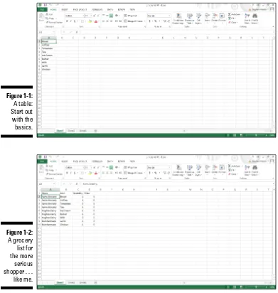
A table is, well, a list. This definition sounds simplistic, I guess. But take a look at the simple table shown in Figure 1-1. This table shows the items that you might shop for at a grocery store on the way home from work.
As I mention in the Introduction of this book, many of the Excel workbooks that you see in the figures of this book are available for download from this book’s companion website. For more on how to access the companion website, see the Introduction.
10
Part I: Where’s the Beef?
Figure 1-1:
A table: Start out with the basics.
Figure 1-2:
A grocery list for the more serious shopper . . .
like me.
11
Chapter 1: Introducing Excel Tables
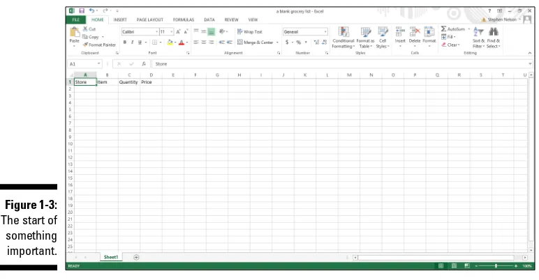
Let me make a handful of observations about the table shown in Figure 1-2. First, each column shows a particular sort of information. In the parlance of database design, each column represents a field. Each field stores the same sort of information. Column A, for example, shows the store where some item can be purchased. (You might also say that this is the Store field.) Each piece of information shown in column A — the Store field — names a store: Sams Grocery, Hughes Dairy, and Butchermans.
The first row in the Excel worksheet provides field names. For example, in Figure 1-2, row 1 names the four fields that make up the list: Store, Item, Quantity, and Price. You always use the first row, called the header row, of an Excel list to name, or identify, the fields in the list.
Starting in row 2, each row represents a record, or item, in the table. A record
is a collection of related fields. For example, the record in row 2 in Figure 1-2 shows that at Sams Grocery, you plan to buy two loaves of bread for a price of $1 each. (Bear with me if these sample prices are wildly off; I usually don’t do the shopping in my household.)
Row 3 shows or describes another item, coffee, also at Sams Grocery, for $8. In the same way, the other rows of the super-sized grocery list show items that you will buy. For each item, the table identifies the store, the item, the quantity, and the price.
Something to understand about Excel tables
An Excel table is a flat-file database. That
flat-file-ish-ness means that there’s only one table in the database. And the flat-file-ish-ness also means that each record stores every bit of information about an item.
In comparison, popular desktop database appli-cations such as Microsoft Access are relational
databases. A relational database stores
infor-mation more efficiently. And the most striking way in which this efficiency appears is that you don’t see lots of duplicated or redundant infor-mation in a relational database. In a relational database, for example, you might not see Sams
Grocery appearing in cells A2, A3, A4, and A5. A relational database might eliminate this redun-dancy by having a separate table of grocery stores.
12
Part I: Where’s the Beef?
Building Tables
You build a table that you want to later analyze by using Excel in one of two ways:
✓ Export the table from a database.
✓ Manually enter items into an Excel workbook.
Exporting from a database
The usual way to create a table to use in Excel is to export information from a database. Exporting information from a database isn’t tricky. However, you need to reflect a bit on the fact that the information stored in your database is probably organized into many separate tables that need to be combined into a large flat-file database or table.
In Chapter 2, I describe the process of exporting data from the database and then importing this data into Excel so it can be analyzed. Hop over to that chapter for more on creating a table by exporting and then importing.
Even if you plan to create your tables by exporting data from a database, however, read on through the next paragraphs of this chapter. Understanding the nuts and bolts of building a table makes exporting database information to a table and later using that information easier.
Building a table the hard way
The other common way to create an Excel table (besides exporting from a relational database) is to do it manually. For example, you can create a table in the same way that I create the grocery list shown in Figure 1-2. You first enter field names into the first row of the worksheet and then enter individual records, or items, into the subsequent rows of the worksheet. When a table isn’t too big, this method is very workable. This is the way, obviously, that I created the table shown in Figure 1-2.
Building a table the semi-hard way
13
Chapter 1: Introducing Excel Tables
Manually adding records into a table
To manually create a list by using the Table command, follow these steps:
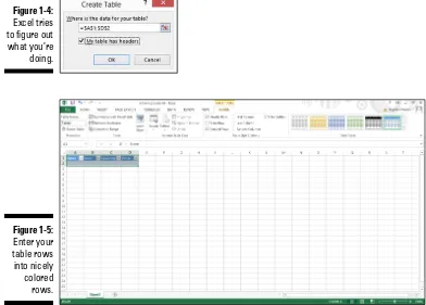
1. Identify the fields in your list.
To identify the fields in your list, enter the field names into row 1 in a blank Excel workbook. For example, Figure 1-3 shows a workbook fragment. Cells A1, B1, C1, and D1 hold field names for a simple grocery list.
Figure 1-3:
The start of something important.
2. Select the Excel table.
The Excel table must include the row of the field names and at least one other row. This row might be blank or it might contain data. In Figure 1-3, for example, you can select an Excel list by dragging the mouse from cell A1 to cell D2.
3. Click the Insert tab and then its Table button to tell Excel that you want to get all official right from the start.
14
Part I: Where’s the Beef?
Figure 1-4:
Excel tries to figure out what you’re doing.
Figure 1-5:
Enter your table rows into nicely colored rows.
4. Describe each record.
To enter a new record into your table, fill in the next empty row. For example, use the Store text box to identify the store where you purchase each item. Use the — oh, wait a minute here. You don’t need me to tell you that the store name goes into the Store column, do you? You can figure that out. Likewise, you already know what bits of information go into the Item, Quantity, and Price column, too, don’t you? Okay. Sorry.
5. Store your record in the table.
15
Chapter 1: Introducing Excel Tables
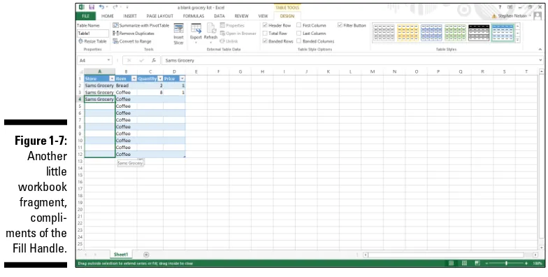
Some table-building tools
Excel includes an AutoFill feature, which is particularly relevant for table building. Here’s how AutoFill works: Enter a label into a cell in a column where it’s already been entered before, and Excel guesses that you’re entering the same thing again. For example, if you enter the label Sams Grocery in cell A2 and then begin to type Sams Grocery in cell A3, Excel guesses that you’re entering Sams Grocery again and finishes typing the label for you. All you need to do to accept Excel’s guess is press Enter. Check it out in Figure 1-6.
Figure 1-6:
A little workbook fragment, compliments of AutoFill.
16
Part I: Where’s the Beef?
Figure 1-7:
Another little workbook fragment, compli-ments of the
Fill Handle.
Analyzing Table Information
Excel provides several handy, easy-to-use tools for analyzing the information that you store in a table. Some of these tools are so easy and straightforward that they provide a good starting point.
Simple statistics
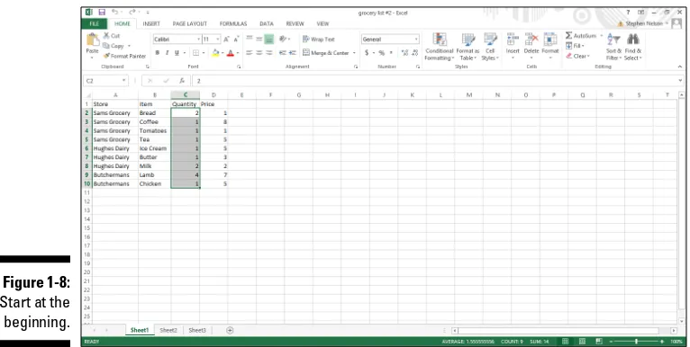
Look again at the simple grocery list table that I mention earlier in the section, “What Is a Table and Why Do I Care?” See Figure 1-8 for this grocery list as I use this information to demonstrate some of the quick-and-dirty statistical tools that Excel provides.
One of the slickest and quickest tools that Excel provides is the ability to effortlessly calculate the sum, average, count, minimum, and maximum of values in a selected range. For example, if you select the range C2 to C10 in Figure 1-8, Excel calculates an average, counts the values, and even sums the quantities, displaying this useful information in the status bar. In Figure 1-8, note the information on the status bar (the lower edge of the workbook):
17
Chapter 1: Introducing Excel Tables
This indicates that the average order quantity is (roughly) 1.5, that you’re shopping for 9 different items, and that the grocery list includes 14 items: Two loaves of bread, one can of coffee, one tomato, one box of tea, and so on.
Figure 1-8:
Start at the beginning.
The big question here, of course, is whether, with 9 different products but a total count of 14 items, you’ll be able to go through the express checkout line. But that information is irrelevant to our discussion. (You, however, might want to acquire another book I’m planning, Grocery Shopping For Dummies.)
You aren’t limited, however, to simply calculating averages, counting entries, and summing values in your list. You can also calculate other statistical measures.
18
Part I: Where’s the Beef?
Table 1-1 Quick Statistical Measures Available on the Status Bar
Option What It DoesCount Tallies the cells that hold labels, values, or formulas. In other words, use this statistical measure when you want to count the number of cells that are not empty.
Count Numerical
Tallies the number of cells in a selected range that hold values or formulas.
Maximum Finds the largest value in the selected range. Minimum Finds the smallest value in the selected range. Sum Adds up the values in the selected range.
No kidding, these simple statistical measures are often all you need to gain wonderful insights into data that you collect and store in an Excel table. By using the example of a simple, artificial grocery list, the power of these quick statistical measures doesn’t seem all that earthshaking. But with real data, these measures often produce wonderful insights.
In my own work as a technology writer, for example, I first noticed the deflation in the technology bubble a decade ago when the total number of computer books that one of the larger distributors sold — information that appeared in an Excel table — began dropping. Sometimes, simply adding, counting, or averaging the values in a table gives extremely useful insights.
Sorting table records
After you place information in an Excel table, you’ll find it very easy to sort the records. You can use the Sort & Filter button’s commands.
Using the Sort buttons
To sort table information by using a Sort & Filter button’s commands, click in the column you want to use for your sorting. For example, to sort a grocery list like the one shown in Figure 1-8 by the store, click a cell in the Store column.
19
Chapter 1: Introducing Excel Tables
Using the Custom Sort dialog box
When you can’t sort table information exactly the way you want by using the Sort A to Z and Sort Z to A commands, use the Custom Sort command.
To use the Custom Sort command, follow these steps:
1. Click a cell inside the table.
2. Click the Sort & Filter button and choose the Sort command from the Sort & Filter menu.
Excel displays the Sort dialog box, as shown in Figure 1-9.
In Excel 2007 and Excel 2010, choose the Data➪Custom Sort command to display the Sort dialog box.
Figure 1-9:
Set sort parameters here.
3. Select the first sort key.
Use the Sort By drop-down list to select the field that you want to use for sorting. Next, choose what you want to use for sorting: values, cell colors, font colors, or icons. Probably, you’re going to sort by values, in which case, you’ll also need to indicate whether you want records arranged in ascending or descending order by selecting either the ascending A to Z or descending Z to A entry from the Order box. Ascending order, predict-ably, alphabetizes labels and arranges values in smallest-value-to-largest-value order. Descending order arranges labels in reverse alphabetical order and values in largest-value-to-smallest-value order. If you sort by color or icons, you need to tell Excel how it should sort the colors by using the options that the Order box provides.
20
Part I: Where’s the Beef?
4. (Optional) Specify any secondary keys.
If you want to sort records that have the same primary key with a second-ary key, click the Add Level button and then use the next row of choices from the Then By drop-down lists to specify which secondary keys you want to use. If you add a level that you later decide you don’t want or need, click the sort level and then click the Delete Level button. You can also duplicate the selected level by clicking Copy Level. Finally, if you do create multiple sorting keys, you can move the selected sort level up or down in significance by clicking the Move Up or Move Down buttons. Note: The Sort dialog box also provides a My Data Has Headers check
box that enables you to indicate whether the worksheet range selection includes the row and field names. If you’ve already told Excel that a work-sheet range is a table, however, this check box is disabled.
5. (Really optional) Fiddle-faddle with the sorting rules.
If you click the Options button in the Sort dialog box, Excel displays the Sort Options dialog box, shown in Figure 1-10. Make choices here to further specify how the first key sort order works.
Figure 1-10:
Sorting out your sorting options.
For a start, the Sort Options dialog box enables you to indicate whether case sensitivity (uppercase versus lowercase) should be considered. You can also use the Sort Options dialog box to tell Excel that it should
sort rows instead of columns or columns instead of rows. You make this specification by using either Orientation radio button: Sort Top to Bottom or Sort Left to Right. Click OK when you’ve sorted out your sort-ing options.
6. Click OK.
21
Chapter 1: Introducing Excel Tables
Using AutoFilter on a table
Excel provides an AutoFilter command that’s pretty cool. When you use AutoFilter, you produce a new table that includes a subset of the records from your original table. For example, in the case of a grocery list table, you could use AutoFilter to create a subset that shows only those items that you’ll purchase at Butchermans or a subset table that shows only those items that cost more than, say, $2.
To use AutoFilter on a table, take these steps:
1. Select your table.
Select your table by clicking one of its cells. By the way, if you haven’t yet turned the worksheet range holding the table data into an “official” Excel table, select the table and then choose the Insert tab’s Table command.
2. (Perhaps unnecessary) Choose the AutoFilter command.
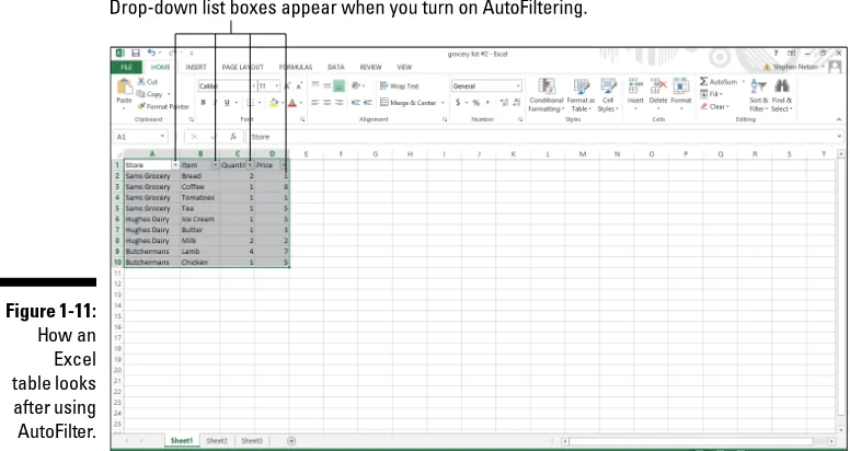
When you tell Excel that a particular worksheet range represents a table, Excel turns the header row, or row of field names, into drop-down lists. Figure 1-11 shows this. If your table doesn’t include these drop-down lists, add them by clicking the Sort & Filter button and choosing the Filter command. Excel turns the header row, or row of field names, into drop-down lists.
Tip: In Excel 2007 and Excel 2010, you choose the Data➪Filter command to tell Excel you want to AutoFilter.
Figure 1-11:
22
Part I: Where’s the Beef?
3. Use the drop-down lists to filter the list.
Each of the drop-down lists that now make up the header row can be used to filter the list.
To filter the list by using the contents of some field, select (or open) the drop-down list for that field. For example, in the case of the little workbook shown in Figure 1-11, you might choose to filter the grocery list so that it shows only those items that you’ll purchase at Sams Grocery. To do this, click the Store drop-down list down-arrow button. When you do, Excel displays a menu of table sorting and filtering options. To see just those records that describe items you’ve purchased at Sams Grocery, select Sams Grocery. Figure 1-12 shows the filtered list with just the Sams Grocery items visible.
If your eyes work better than mine do, you might even be able to see a little picture of a funnel on the Store column’s drop-down list button. This icon tells you the table is filtered using the Store columns data.
Figure 1-12:
Sams and Sams alone.
To unfilter the table, open the Store drop-down list and choose Select All. If you’re filtering a table using the table menu, you can also sort the
23
Chapter 1: Introducing Excel Tables
Undoing a filter
To remove an AutoFilter, display the table menu by clicking a drop-down list’s button. Then choose the Clear Filter command from the table menu.
Turning off filter
The AutoFilter command is actually a toggle switch. When filtering is turned on, Excel turns the header row of the table into a row of drop-down lists. When you turn off filtering, Excel removes the drop-down list functionality. To turn off filtering and remove the Filter drop-down lists, simply click the Sort & Filter button and choose the Filter command (or in Excel 2007 or Excel 2010, choose Data➪Filter command).
Using the custom AutoFilter
You can also construct a custom AutoFilter. To do this, select the Text Filter command from the table menu and choose one of its text filtering options. No matter which text filtering option you pick, Excel displays the Custom AutoFilter dialog box, as shown in Figure 1-13. This dialog box enables you to specify with great precision what records you want to appear on your filtered list.
Figure 1-13:
The Custom AutoFilter dialog box.
To create a custom AutoFilter, take the following steps:
1. Turn on the Excel Filters.
24
Part I: Where’s the Beef?
2. Select the field that you want to use for your custom AutoFilter.
To indicate which field you want to use, open the filtering drop-down list for that field to display the table menu, select Text Filters, and then select a filtering option. When you do this, Excel displays the Custom AutoFilter dialog box. (Refer to Figure 1-13.)
3. Describe the AutoFilter operation.
To describe your AutoFilter, you need to identify (or confirm) the filtering operation and the filter criteria. Use the left-side set of drop-down lists to select a filtering option. For example, in Figure 1-14, the filtering option selected in the first Custom AutoFilter set of dialog boxes is Begins With. If you open this drop-down list, you’ll see that Excel provides a series of filtering options:
• Begins With • Equals
• Does Not Equal
• Is Greater Than or Equal To • Is Less Than
• Is Less Than or Equal To • Begins With
• Does Not Begin With • Ends With
• Does Not End With • Contains
• Does Not Contain
The key thing to be aware of is that you want to pick a filtering operation that, in conjunction with your filtering criteria, enables you to identify the records that you want to appear in your filtered list. Note that Excel initially fills in the filtering option that matches the command you selected on the Text Filter submenu, but you can change this initial filtering selection to something else.
25
Chapter 1: Introducing Excel Tables
4. Describe the AutoFilter filtering criteria.
After you pick the filtering option, you describe the filtering criteria by using the right-hand drop-down list. For example, if you want to filter records that equal Sams Grocery or, more practically, that begin with the word Sams, you enter Sams into the right-hand box. Figure 1-14 shows this custom AutoFilter criterion.
You can use more than one AutoFilter criterion. If you want to use two custom AutoFilter criteria, you need to indicate whether the criteria are both applied together or are applied independently. You select either the And or Or radio button to make this specification.
5. Click OK.
Excel then filters your table according to your custom AutoFilter.
Figure 1-14:
Setting up a custom AutoFilter.
Filtering a filtered table
You can filter a filtered table. What this often means is that if you want to build a highly filtered table, you will find your work easiest if you just apply several sets of filters.
If you want to filter the grocery list to show only the most expensive items that you purchase at Sams Grocery, for example, you might first filter the table to show items from Sams Grocery only. Then, working with this filtered table, you would further filter the table to show the most expensive items or only those items with the price exceeding some specified amount.
26
Part I: Where’s the Beef?
Building on the earlier section “Using the custom AutoFilter,” I want to make this important point: Although the Custom AutoFilter dialog box does enable you to filter a list based on two criteria, sometimes filtering operations apply to the same field. And if you need to apply more than two filtering operations to the same field, the only way to easily do this is to filter a filtered table.
Using advanced filtering
Most of the time, you’ll be able to filter table records in the ways that you need by using the Filter command or that unnamed table menu of filtering options. However, in some cases, you might want to exert more control over the way filtering works. When this is the case, you can use the Excel advanced filters.
Writing Boolean expressions
Before you can begin to use the Excel advanced filters, you need to know how to construct Boolean logic expressions. For example, if you want to filter the grocery list table so that it shows only those items that cost more than $1 or those items with an extended price of more than $5, you need to know how to write a Boolean logic, or algebraic, expression that describes the condition in which the price exceeds $1 or the extended price exceeds or equals $5.
27
Chapter 1: Introducing Excel Tables
To construct a Boolean expression, you use a comparison operator from Table 1-2 and then a value used in the comparison.
Table 1-2
Boolean Logic
Operator What It Does
= Equals
< Is less than
<= Is less than or equal to > Is greater than
>= Is greater than or equal to <> Is not equal to
In Figure 1-15, for example, the Boolean expression in cell A14 (>1), checks to see whether a value is greater than 1, and the Boolean expression in cell B14 (>=5) checks to see whether the value is greater than or equal to 5. Any record that meets both of these tests gets included by the filtering operation.
Here’s an important point: Any record in the table that meets the criteria in
any one of the criteria rows gets included in the filtered table. Accordingly, if you want to include records for items that either cost more than $1 apiece
or that totaled at least $5 in shopping expense (after multiplying the quantity times the unit price), you use two rows — one for each criterion. Figure 1-16 shows how you would create a worksheet that does this.
Figure 1-16:
A work-sheet with
28
Part I: Where’s the Beef?
Running an advanced filter operation
After you set up a table for an advanced filter and the criteria range — what I did in Figures 1-15 and 1-16 — you’re ready to run the advanced filter operation. To do so, take these steps:
1. Select the table.
To select the table, drag the mouse from the top-left corner of the list to the lower-right corner. You can also select an Excel table by selecting the cell in the top-left corner, holding down the Shift key, pressing the End key, pressing the right arrow, pressing the End key, and pressing the down arrow. This technique selects the Excel table range using the arrow keys.
2. Choose Data tab’s Advanced Filter.
Excel displays the Advanced Filter dialog box, as shown in Figure 1-17.
Figure 1-17:
Set up an advanced filter here.
3. Tell Excel where to place the filtered table.
Use either Action radio button to specify whether you want the table filtered in place or copied to some new location. You can either filter the table in place (meaning Excel just hides the records in the table that don’t meet the filtering criteria), or you can copy the records that meet the filtering criteria to a new location.
4. Verify the list range.
The worksheet range shown in the List Range text box — $A$1:$E$10 in Figure 1-17 — should correctly identify the list. If your text box doesn’t show the correct worksheet range, however, enter it. (Remember how I said earlier in the chapter that Excel used to call these tables “lists”? Hence the name of this box.)
29
Chapter 1: Introducing Excel Tables
6. (Optional) If you’re copying the filtering results, provide the destination.
If you tell Excel to copy the filter results to some new location, use the Copy To text box to identify this location.
7. Click OK.
Excel filters your list . . . I mean table. Figure 1-18 shows what the filtered list looks like. Note that the table now shows only those items that cost more than $1 and on which the extended total equals or exceeds $5.
Figure 1-18:
The now-filtered results.
Chapter 2
Grabbing Data from
External Sources
In This Chapter
▶ Exporting data from other programs
▶ Importing data into Excel
▶ Running a web query
▶ Importing a database table
▶ Querying an external database
I
n many cases, the data that you want to analyze with Excel resides in an external database or in a database application, such as a corporate accounting system. Thus, often your very first step and very first true chal-lenge are to get that data into an Excel workbook and in the form of an Excel table.You can use two basic approaches to grab the external data that you want to analyze. You can export data from another program and then import that data into Excel, or you can query a database directly from Excel. I describe both approaches in this chapter.
Getting Data the Export-
Import Way
32
Part I: Where’s the Beef?
Exporting: The first step
Your first step when grabbing data from one of these external sources, assuming that you want to later import the data, is to first use the other application program — such as an accounting program — to export the to-be-analyzed data to a file.
You have two basic approaches available for exporting data from another application: direct exporting and exporting to a text file.
Direct exporting
Direct exporting is available in many accounting programs because accoun-tants love to use Excel to analyze data. For example, the most popular small business accounting program in the world is QuickBooks from Intuit. When you produce an accounting report in QuickBooks, the report docu-ment window includes a button labeled Excel or Export. Click this button, and QuickBooks displays the Send Report to Excel dialog box, as shown in Figure 2-1.
Figure 2-1:
Begin exporting here.
The Send Report to Excel dialog box provides radio buttons with which you indicate whether you want to send the report to a comma-separated-values file, to a new Excel spreadsheet, or to an existing Excel spreadsheet.
33
Chapter 2: Grabbing Data from External Sources
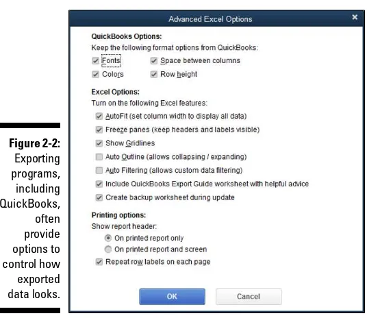
The Export Report dialog box also includes an Advanced button. Click this button, and QuickBooks displays the Advanced dialog box (see Figure 2-2) that you can use to control how the exported report looks. For example, you get to pick which fonts, colors, spacing, and row height that you want. You also get to turn on and turn off Excel features in the newly created workbook, including AutoFit, Gridlines, and so on.
Figure 2-2:
Exporting programs, including QuickBooks, often provide options to control how exported data looks.
In Figure 2-3, you can see how the QuickBooks report looks after it has been directly exported to Excel.
Okay, obviously, you might not want to export from QuickBooks. You might have other applications that you want to export data from. You can export data directly from a database program like Microsoft Access, for example. But the key thing that you need to know — and the reason that I discuss in detail how QuickBooks works — is that applications that store and collect data often provide a convenient way for you to export information to Excel. Predictably, some application programs work differently, but usually, the process is little more than clicking a button labeled Excel (as is the case in QuickBooks) or choosing a command labeled something like Export or Export to Excel.
34
Part I: Where’s the Beef?
Figure 2-3: A QuickBooks report that has been directly exported to Excel.
Versions of Microsoft Access up through and including Access 2003 include an Export command on the File menu, and Access 2007 and later versions include an Export command on its Microsoft Office menu. Choose the Export command to export an Access table, report, or query to Excel. Just choose the appropriate command and then use the dialog box that Access displays to specify where the exported information should be placed.
Exporting to a text file
When you need to export data first to a text file because the other applica-tion won’t automatically export your data to an Excel workbook, you need to go to a little more effort. Fortunately, the process is still pretty darn straightforward.
When you work with applications that won’t automatically create an Excel workbook, you just create a text version of a report that shows the data that you want to analyze. For example, to analyze sales of items that your firm makes, you first create a report that shows this.
The trick is that you send the report to a text file rather than sending this report to a printer. This way, the report gets stored on disk as text rather than printed. Later, Excel can easily import these text files.
35
Chapter 2: Grabbing Data from External Sources
Figure 2-4:
Begin to export a text file from a QuickBooks report.
The next step is to print this report to a text file. In QuickBooks, you click the Print button or choose File➪Print Report. Using either approach, QuickBooks displays the Print Reports dialog box, as shown in Figure 2-5.
Figure 2-5:
Print a QuickBooks report here.
36
Part I: Where’s the Beef?
If you want to later import the information on the report, you should print the report to a file. In the case of QuickBooks, this means that you select the File radio button. (Refer to Figure 2-5.)
The other thing that you need to do — if you’re given a choice — is to use a delimiter. In Figure 2-5, the File drop-down list shows ASCII text file as the type of file that QuickBooks will print. Often, though, applica-tions — including QuickBooks — let you print delimited text files.
Delimited text files use standard characters, called delimiters, to separate fields of information in the report. You can still import a straight ASCII text file, but importing a delimited text file is easier. Therefore, if your other program gives you the option of creating delimited text files, do so. In QuickBooks, you can create both comma-delimited files and tab-delimited files.
In QuickBooks, you indicate that you want a delimited text file by choosing Comma Delimited File or Tab Delimited File from the File drop-down list of the Print Reports dialog box.
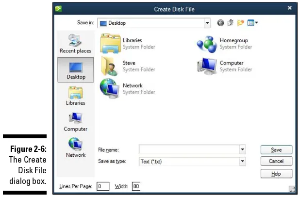
To print the report as a file, you simply click the Print button of the Print Reports dialog box. Typically, the application (QuickBooks, in this example) prompts you for a pathname, like in the Create Disk File dialog box shown in Figure 2-6. The pathname includes both the drive and folder location of the text file as well as the name of the file. You provide this information, and then the application produces the text file . . . or hopefully, the delimited text file. And that’s that.
Figure 2-6:
37
Chapter 2: Grabbing Data from External Sources
Importing: The second
step (if necessary)
When you don’t or can’t export directly to Excel, you need to take the second step of importing the ASCII text file that you created with the other program. (To read more about exporting to a text file, see the preceding section.)
To import the ASCII text file, first open the text file itself from within Excel. When you open the text file, Excel starts the Text Import Wizard. This wizard walks you through the steps to describe how information in a text file should be formatted and rearranged as it’s placed in an Excel workbook.
One minor wrinkle in this importing business is that the process works differ-ently depending on whether you’re importing straight (ASCII) text or delim-ited text.
Importing straight text
Here are the steps that you take to import a straight text file:
1. Open the text file by choosing Open from the File menu or by choosing the Data tab’s Get External Data from Text command.
Excel displays the Open dialog box, shown in Figure 2-7, if you choose the Open command. Excel displays a nearly identical Import Text File dialog box if you choose the Data tab’s Get External Data from Text command.
Figure 2-7:
38
Part I: Where’s the Beef?
2. Choose Text Files from the drop-down list that appears to the right of the File text box.
3. Use the Look In drop-down list to identify the folder in which you placed the exported text file.
You should see the text file listed in the Open dialog box.
4. To open the text file, double-click its icon.
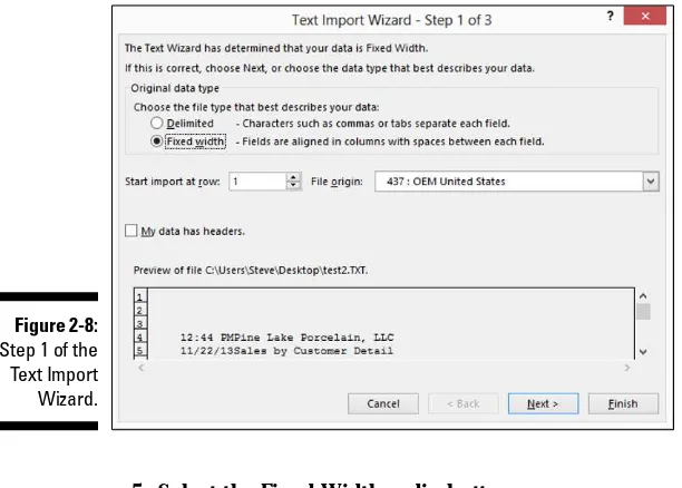
Excel starts the Text Import Wizard, as shown in Figure 2-8.
Figure 2-8:
Step 1 of the Text Import Wizard.
5. Select the Fixed Width radio button.
This tells Excel that the fields in the text file are arranged in evenly spaced columns.
6. In the Start Import at Row text box, identify the row in the ASCII text file that should be the first row of the spreadsheet.
In general, ASCII text files use the first several rows of the file to show report header information. For this reason, you typically won’t want to start importing at row 1; you’ll want to start importing at row 10 or 20 or 5. Don’t get too tense about this business of telling the Text Import Wizard
39
Chapter 2: Grabbing Data from External Sources
7. Click Next.
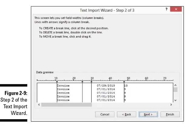
Excel displays the second step dialog box of the Text Import Wizard, as shown in Figure 2-9. You use this second Text Import Wizard dialog box to break the rows of the text files into columns.
You might not need to do much work identifying where rows should be broken into columns. Excel, after looking carefully at the data in the to-be-imported text file, suggests where columns should be broken and draws vertical lines at the breaks.
Figure 2-9:
Step 2 of the Text Import Wizard.
8. In the Data Preview section of the second wizard dialog box, review the text breaks and amend them as needed.
• If they’re incorrect, drag the break lines to a new location.
• To remove a break, double-click the break line.
• To create or add a new break, click at the point where you want the break to occur.
9. Click Next.