Excel
®
2007
FOR
by Greg Harvey, PhD
Excel
®
2007
FOR
111 River Street Hoboken, NJ 07030-5774
www.wiley.com
Copyright © 2007 by Wiley Publishing, Inc., Indianapolis, Indiana Published by Wiley Publishing, Inc., Indianapolis, Indiana Published simultaneously in Canada
No part of this publication may be reproduced, stored in a retrieval system or transmitted in any form or by any means, electronic, mechanical, photocopying, recording, scanning or otherwise, except as permit-ted under Sections 107 or 108 of the 1976 Unipermit-ted States Copyright Act, without either the prior written permission of the Publisher, or authorization through payment of the appropriate per-copy fee to the Copyright Clearance Center, 222 Rosewood Drive, Danvers, MA 01923, (978) 750-8400, fax (978) 646-8600. Requests to the Publisher for permission should be addressed to the Legal Department, Wiley Publishing, Inc., 10475 Crosspoint Blvd., Indianapolis, IN 46256, (317) 572-3447, fax (317) 572-4355, or online at
http://www.wiley.com/go/permissions.
Trademarks:Wiley, the Wiley Publishing logo, For Dummies, the Dummies Man logo, A Reference for the Rest of Us!, The Dummies Way, Dummies Daily, The Fun and Easy Way, Dummies.com, and related trade dress are trademarks or registered trademarks of John Wiley & Sons, Inc. and/or its affiliates in the United States and other countries, and may not be used without written permission. Microsoft is a registered trademark or trademark of Microsoft Corporation. All other trademarks are the property of their respec-tive owners. Wiley Publishing, Inc., is not associated with any product or vendor mentioned in this book.
LIMIT OF LIABILITY/DISCLAIMER OF WARRANTY: WHILE THE PUBLISHER AND AUTHOR HAVE USED THEIR BEST EFFORTS IN PREPARING THIS BOOK, THEY MAKE NO REPRESENTATIONS OR WAR-RANTIES WITH RESPECT TO THE ACCURACY OR COMPLETENESS OF THE CONTENTS OF THIS BOOK AND SPECIFICALLY DISCLAIM ANY IMPLIED WARRANTIES OF MERCHANTABILITY OR FITNESS FOR A PARTICULAR PURPOSE. NO WARRANTY MAY BE CREATED OR EXTENDED BY SALES REPRESENTA-TIVES OR WRITTEN SALES MATERIALS. THE ADVICE AND STRATEGIES CONTAINED HEREIN MAY NOT BE SUITABLE FOR YOUR SITUATION. YOU SHOULD CONSULT WITH A PROFESSIONAL WHERE APPRO-PRIATE. NEITHER THE PUBLISHER NOR AUTHOR SHALL BE LIABLE FOR ANY LOSS OF PROFIT OR ANY OTHER COMMERCIAL DAMAGES, INCLUDING BUT NOT LIMITED TO SPECIAL, INCIDENTAL, CON-SEQUENTIAL, OR OTHER DAMAGES.
For general information on our other products and services or to obtain technical support, please contact our Customer Care Department within the U.S. at 800-762-2974, outside the U.S. at 317-572-3993, or fax 317-572-4002.
Wiley also publishes its books in a variety of electronic formats. Some content that appears in print may not be available in electronic books.
Library of Congress Control Number: 2006934835 ISBN-13: 978-0-470-03737-9
ISBN-10: 0-470-03737-7 1B/QV/RS/QW/IN
Greg Harveyhas authored tons of computer books, the most recent being Excel Workbook For Dummiesand Roxio Easy Media Creator 8 For Dummies, and the most popular being Excel 2003 For Dummiesand Excel 2003 All-In-One Desk Reference For Dummies. He started out training business users on how to use IBM personal computers and their attendant computer software in the rough and tumble days of DOS, WordStar, and Lotus 1-2-3 in the mid-80s of the last century. After working for a number of independent training firms, Greg went on to teach semester-long courses in spreadsheet and database management software at Golden Gate University in San Francisco.
His love of teaching has translated into an equal love of writing. For Dummies books are, of course, his all-time favorites to write because they enable him to write to his favorite audience: the beginner. They also enable him to use humor (a key element to success in the training room) and, most delightful of all, to express an opinion or two about the subject matter at hand.
An Erucolindo melindonya
Author’s Acknowledgments
Let me take this opportunity to thank all the people, both at Wiley Publishing, Inc., and at Mind over Media, Inc., whose dedication and talent combined to get this book out and into your hands in such great shape.
At Wiley Publishing, Inc., I want to thank Andy Cummings and Katie Feltman for their encouragement and help in getting this project underway and their ongoing support every step of the way, and project editor Christine Berman. These people made sure that the project stayed on course and made it into production so that all the talented folks on the production team could create this great final product.
Some of the people who helped bring this book to market include the following:
Acquisitions, Editorial, and Media Development
Project Editor:Christine Berman
Senior Acquisitions Editor:Katie Feltman Copy Editor:Christine Berman
Technical Editor:Gabrielle Sempf Editorial Manager:Jodi Jensen Media Development Manager: Laura Carpenter VanWinkle Editorial Assistant:Amanda Foxworth
Cartoons:Rich Tennant (www.the5thwave.com)
Production
Project Coordinator: Adrienne Martinez Layout and Graphics: Stephanie D. Jumper,
Barbara Moore, Barry Offringa, Heather Ryan
Proofreaders: John Greenough, Jessica Kramer, Techbooks Indexer: Techbooks
Anniversary Logo Design:Richard Pacifico
Publishing and Editorial for Technology Dummies
Richard Swadley,Vice President and Executive Group Publisher Andy Cummings,Vice President and Publisher
Mary C. Corder,Editorial Director Publishing for Consumer Dummies
Diane Graves Steele,Vice President and Publisher Joyce Pepple,Acquisitions Director
Composition Services
Introduction ...1
Part I: Getting In on the Ground Floor ...9
Chapter 1: The Excel 2007 User Experience ...11
Chapter 2: Creating a Spreadsheet from Scratch ...51
Part II: Editing Without Tears...97
Chapter 3: Making It All Look Pretty ...99
Chapter 4: Going through Changes ...141
Chapter 5: Printing the Masterpiece ...173
Part III: Getting Organized and Staying That Way ...201
Chapter 6: Maintaining the Worksheet ...203
Chapter 7: Maintaining Multiple Worksheets ...231
Part IV: Digging Data Analysis...253
Chapter 8: Doing What-If Analysis...255
Chapter 9: Playing with Pivot Tables ...269
Part V: Life Beyond the Spreadsheet ...285
Chapter 10: Charming Charts and Gorgeous Graphics ...287
Chapter 11: Getting on the Data List...319
Chapter 12: Hyperlinks and Macros...343
Part VI: The Part of Tens ...355
Chapter 13: Top Ten New Features in Excel 2007...357
Chapter 14: Top Ten Beginner Basics ...361
Chapter 15: The Ten Commandments of Excel 2007...363
Introduction...1
About This Book...1
How to Use This Book ...2
What You Can Safely Ignore ...2
Foolish Assumptions ...3
How This Book Is Organized...3
Part I: Getting In on the Ground Floor ...3
Part II: Editing Without Tears...4
Part III: Getting Organized and Staying That Way ...4
Part IV: Digging Data Analysis...4
Part V: Life Beyond the Spreadsheet ...4
Part VI: The Part of Tens ...5
Conventions Used in This Book ...5
Keyboard and mouse ...5
Special icons ...7
Where to Go from Here...8
Part I: Getting In on the Ground Floor ...9
Chapter 1: The Excel 2007 User Experience . . . .11
Excel’s Ribbon User Interface...12
Manipulating the Office Button ...12
Bragging about the Ribbon ...14
Adapting the Quick Access toolbar ...18
Having fun with the Formula bar...21
What to do in the Worksheet area...22
Showing off the Status bar ...27
Starting and Exiting Excel ...29
Starting Excel from the Windows Vista Start menu ...29
Starting Excel from the Windows XP Start menu ...29
Pinning Excel to the Start menu ...30
Creating an Excel desktop shortcut for Windows Vista ...30
Creating an Excel desktop shortcut for Windows XP ...31
Adding the Excel desktop shortcut to the Quick Launch toolbar ...32
Exiting Excel ...32
Help Is on the Way ...33
Migrating to Excel 2007 from Earlier Versions ...34
Cutting the Ribbon down to size ...35
Finding the Formatting Toolbar buttons equivalents...43
Putting the Quick Access toolbar to excellent use ...45
Getting good to go with Excel 2007...49
Chapter 2: Creating a Spreadsheet from Scratch . . . .51
So What Ya Gonna Put in That New Workbook of Yours? ...52
The ins and outs of data entry...52
You must remember this . . . ...53
Doing the Data-Entry Thing ...53
It Takes All Types ...56
The telltale signs of text ...56
How Excel evaluates its values...58
Fabricating those fabulous formulas! ...64
If you want it, just point it out ...67
Altering the natural order of operations ...67
Formula flub-ups...68
Fixing Up Those Data Entry Flub-Ups...70
You really AutoCorrect that for me...70
Cell editing etiquette...71
Taking the Drudgery out of Data Entry ...73
I’m just not complete without you ...73
Fill ’er up with AutoFill ...75
Inserting special symbols...80
Entries all around the block...81
Data entry express ...82
How to Make Your Formulas Function Even Better...83
Inserting a function into a formula with the Function Wizard button ...84
Editing a function with the Function Wizard button...87
I’d be totally lost without AutoSum ...87
Making Sure That the Data Is Safe and Sound ...90
The Save As dialog box in Windows Vista...91
The Save As dialog box in Windows XP...92
Changing the default file location ...93
The difference between the XLSX and XLS file format ...94
Saving the Workbook as a PDF File ...95
Document Recovery to the Rescue ...96
Part II: Editing Without Tears ...97
Chapter 3: Making It All Look Pretty . . . .99
Choosing a Select Group of Cells ...100
Point-and-click cell selections ...100
Keyboard cell selections ...104
Cell Formatting from the Home Tab ...109
Formatting Cells Close to the Source with the Mini Toolbar...113
Using the Format Cells Dialog Box...114
Getting comfortable with the number formats ...114
The values behind the formatting...119
Make it a date!...121
Ogling some of the other number formats...122
Calibrating Columns ...123
Rambling rows ...124
Now you see it, now you don’t ...125
Futzing with the Fonts ...126
Altering the Alignment ...128
Intent on indents ...130
From top to bottom...130
Tampering with how the text wraps ...131
Reorienting cell entries...133
Shrink to fit...134
Bring on the borders! ...135
Applying fill colors, patterns, and gradient effects to cells ...136
Do It in Styles ...138
Creating a new style for the gallery ...138
Copying custom styles from one workbook into another...138
Fooling Around with the Format Painter ...139
Chapter 4: Going through Changes . . . .141
Opening the Darned Thing Up for Editing ...142
The Open dialog box in Excel 2007 running on Windows Vista ...142
The Open dialog box in Excel 2007 running on Windows XP ...144
Opening more than one workbook at a time ...146
Opening recently edited workbooks ...146
When you don’t know where to find them...147
Opening files with a twist ...149
Much Ado about Undo ...150
Undo is Redo the second time around ...150
What ya gonna do when you can’t Undo? ...151
Doing the Old Drag-and-Drop Thing ...151
Copies, drag-and-drop style ...153
Insertions courtesy of drag and drop ...154
Formulas on AutoFill...155
Relatively speaking ...156
Some things are absolutes! ...157
Cut and paste, digital style...159
Paste it again, Sam . . ...160
Keeping pace with the Paste Options...160
Paste it from the Clipboard task pane ...161
Let’s Be Clear about Deleting Stuff...164
Sounding the all clear! ...164
Get these cells outta here!...165
Staying in Step with Insert ...166
Stamping Out Your Spelling Errors ...167
Stamping Out Errors with Text to Speech...169
Chapter 5: Printing the Masterpiece . . . .173
Taking a Gander at the Pages in Page Layout View ...174
Checking the Printout with Print Preview ...175
Printing the Worksheet...177
Printing the Worksheet from the Print Dialog Box ...178
Printing particular parts of the workbook ...179
Setting and clearing the Print Area ...181
My Page Was Set Up! ...181
Using the buttons in the Page Setup group...182
Using the buttons in the Scale to Fit group...188
Using the Print buttons in the Sheet Options group...188
From Header to Footer ...189
Adding an Auto Header or Auto Footer...190
Creating a custom header or footer...192
Solving Page Break Problems ...196
Letting Your Formulas All Hang Out ...198
Part III: Getting Organized and Staying That Way ...201
Chapter 6: Maintaining the Worksheet . . . .203
Zeroing In with Zoom...204
Splitting the Difference ...206
Fixed Headings Courtesy of Freeze Panes ...209
Electronic Sticky Notes ...212
Adding a comment to a cell ...212
Comments in review...214
Editing the comments in a worksheet ...215
Getting your comments in print ...216
The Cell Name Game...216
If I only had a name . . . ...216
Name that formula!...217
Naming constants...218
Seek and Ye Shall Find . . . ...220
You Can Be Replaced! ...223
Do Your Research...224
You Can Be So Calculating ...226
Chapter 7: Maintaining Multiple Worksheets . . . .231
Juggling Worksheets ...232
Sliding between the sheets ...232
Editing en masse...235
Don’t Short-Sheet Me! ...236
A worksheet by any other name . . ...237
A sheet tab by any other color . . . ...238
Getting your sheets in order ...239
Opening Windows on Your Worksheets ...240
Comparing Two Worksheets Side by Side...245
Moving and Copying Sheets to Other Workbooks ...246
To Sum Up . . . ...249
Part IV: Digging Data Analysis ...253
Chapter 8: Doing What-If Analysis . . . .255
Playing what-if with Data Tables ...256
Creating a one-variable data table ...256
Creating a two-variable data table ...259
Playing What-If with Goal Seeking...261
Examining Different Cases with Scenario Manager ...264
Setting up the various scenarios ...264
Producing a summary report...266
Chapter 9: Playing with Pivot Tables . . . .269
Pivot Tables: The Ultimate Data Summary ...269
Producing a Pivot Table ...270
Formatting a Pivot Table ...273
Refining the Pivot Table style ...274
Formatting the values in the pivot table ...275
Sorting and Filtering the Pivot Table Data ...275
Filtering the report ...276
Filtering individual Column and Row fields ...276
Sorting the pivot table ...278
Modifying a Pivot Table...278
Modifying the pivot table fields...278
Pivoting the table’s fields ...279
Modifying the table’s summary function ...280
Get Smart with a Pivot Chart ...281
Moving a pivot chart to its own sheet ...282
Filtering a pivot chart ...283
Part V: Life Beyond the Spreadsheet...285
Chapter 10: Charming Charts and Gorgeous Graphics . . . .287
Making Professional-Looking Charts ...287
Creating a new chart ...288
Moving and resizing an embedded chart in a worksheet ...290
Moving an embedded chart onto its own chart sheet ...290
Customizing the chart type and style from the Design tab ...291
Customizing chart elements from the Layout tab...292
Editing the titles in a chart...295
Formatting chart elements from the Format tab...296
Adding Great Looking Graphics ...299
Telling all with a text box ...300
The wonderful world of Clip Art...302
Inserting pictures from graphics files...305
Editing Clip Art and imported pictures ...305
Formatting Clip Art and imported pictures ...305
Adding preset graphic shapes ...307
Working with WordArt ...308
Make mine SmartArt ...310
Theme for a day...313
Controlling How Graphic Objects Overlap ...314
Reordering the layering of graphic objects ...314
Grouping graphic objects...315
Hiding graphic objects...315
Printing Just the Charts...317
Chapter 11: Getting on the Data List . . . .319
Creating a Data List...319
Adding records to a data list...321
Sorting Records in a Data List ...329
Sorting records on a single field...330
Sorting records on multiple fields...331
Filtering the Records in a Data List...333
Using readymade number filters ...334
Using readymade date filters ...335
Getting creative with custom filtering ...336
Importing External Data ...339
Querying an Access database table...339
Chapter 12: Hyperlinks and Macros . . . .343
Using Add-Ins in Excel 2007 ...343
Adding Hyperlinks to a Worksheet ...345
Automating Commands with Macros ...348
Recording new macros ...348
Running macros...352
Assigning macros to the Quick Access toolbar...353
Part VI: The Part of Tens...355
Chapter 13: Top Ten New Features in Excel 2007 . . . .357
Chapter 14: Top Ten Beginner Basics . . . .361
Chapter 15: The Ten Commandments of Excel 2007 . . . .363
I
’m very proud to present you with the completely revamped and almost totally brand new Excel 2007 For Dummies,the latest version of everybody’s favorite book on Microsoft Office Excel for readers with no intention whatso-ever of becoming spreadsheet gurus. The dramatic changes evident in this version of the book reflect the striking, dare I say, revolutionary changes that Microsoft has brought to its ever-popular spreadsheet program. One look at the new Ribbon command structure and all those rich style galleries in Excel 2007 and you know you’re not in Kansas anymore ‘cause this is definitelynot your mother’s Excel!In keeping with Excel’s more graphical and colorful look and feel, Excel 2007 For Dummieshas taken on some color of its own (just take a gander at those color plates in the mid-section of the book) and now starts off with a defini-tive introduction to the new user Ribbon interface. This chapter is written both for those of you for whom Excel is a completely new experience and those of you who have had some experience with the old pull-down menu and multi-toolbar Excel interface who are now faced with the seemingly daunting task of getting comfortable with a whole new user experience.
Excel 2007 For Dummiescovers all the fundamental techniques you need to know in order to create, edit, format, and print your own worksheets. In addition to showing you around the worksheet, this book also exposes you to the basics of charting, creating data lists, and performing data analysis. Keep in mind, though, that this book just touches on the easiest ways to get a few things done with these features — I make no attempt to cover charting, data lists, or data analysis in the same definitive way as spread-sheets: This book concentrates on spreadsheets because spreadsheets are what most regular folks create with Excel.
About This Book
Each discussion of a topic briefly addresses the question of what a particular feature is good for before launching into how to use it. In Excel, as with most other sophisticated programs, you usually have more than one way to do a task. For the sake of your sanity, I have purposely limited the choices by usu-ally giving you only the most efficient ways to do a particular task. Later on, if you’re so tempted, you can experiment with alternative ways of doing a task. For now, just concentrate on performing the task as I describe.
As much as possible, I’ve tried to make it unnecessary for you to remember anything covered in another section of the book. From time to time, however, you will come across a cross-reference to another section or chapter in the book. For the most part, such cross-references are meant to help you get more complete information on a subject, should you have the time and interest. If you have neither, no problem; just ignore the cross-references as if they never existed.
How to Use This Book
This book is like a reference in which you start out by looking up the topic you need information about (in either the table of contents or the index), and then you refer directly to the section of interest. I explain most topics conver-sationally (as though you were sitting in the back of a classroom where you can safely nap). Sometimes, however, my regiment-commander mentality takes over, and I list the steps you need to take to accomplish a particular task in a particular section.
What You Can Safely Ignore
When you come across a section that contains the steps you take to get something done, you can safely ignore all text accompanying the steps (the text that isn’t in bold) if you have neither the time nor the inclination to wade through more material.
Foolish Assumptions
I’m going to make only one assumption about you (let’s see how close I get): You have access to a PC (at least some of the time) that is running either Windows Vista or Windows XP and on which Microsoft Office Excel 2007 is installed. However, having said that, I make no assumption that you’ve ever launched Excel 2007, let alone done anything with it.
This book is intended ONLY for users of Microsoft Office Excel 2007! If you’re using any previous version of Excel for Windows (from Excel 97 through 2003), the information in this book will only confuse and confound you as your ver-sion of Excel works nothing like the 2007 verver-sion this book describes.
If you are working on an earlier version of Excel, please put this book down slowly and instead pick up a copy of Excel 2003 For Dummies, published by Wiley Publishing.
How This Book Is Organized
This book is organized in six parts (which gives you a chance to see at least six of those great Rich Tennant cartoons!). Each part contains two or more chapters (to keep the editors happy) that more or less go together (to keep you happy). Each chapter is further divided into loosely related sections that cover the basics of the topic at hand. You should not, however, get too hung up on following along with the structure of the book; ultimately, it doesn’t matter at all if you find out how to edit the worksheet before you learn how to format it, or if you figure out printing before you learn editing. The impor-tant thing is that you find the information — and understand it when you find it — when you need to perform a particular task.
In case you’re interested, a synopsis of what you find in each part follows.
Part I: Getting In on the Ground Floor
Part II: Editing Without Tears
In this part, I show how to edit spreadsheets to make them look good, as well as how to make major editing changes to them without courting disaster. Peruse Chapter 3 when you need information on formatting the data to improve the way it appears in the worksheet. See Chapter 4 for rearranging, deleting, or inserting new information in the worksheet. And read Chapter 5 for the skinny on printing out your finished product.
Part III: Getting Organized
and Staying That Way
Here I give you all kinds of information on how to stay on top of the data that you’ve entered into your spreadsheets. Chapter 6 is full of good ideas on how to keep track of and organize the data in a single worksheet. Chapter 7 gives you the ins and outs of working with data in different worksheets in the same workbook and gives you information on transferring data between the sheets of different workbooks.
Part IV: Digging Data Analysis
This part consists of two chapters. Chapter 8 gives you an introduction to performing various types of what-if analysis in Excel, including setting up data tables with one and two inputs, performing goal seeking, and creating different cases with Scenario Manager. Chapter 9 introduces you to Excel’s vastly improved pivot table and pivot chart capabilities that enable you to summarize and filter vast amounts of data in a worksheet table or data list in a compact tabular or chart format.
Part V: Life Beyond the Spreadsheet
Part VI: The Part of Tens
As is the tradition in For Dummiesbooks, the last part contains lists of the top ten most useful and useless facts, tips, and suggestions. In this part, you find three chapters. Chapter 13 provides my top ten list of the best new features in Excel 2007 (and boy was it hard keeping it down to just ten). Chapter 14 gives you the top ten beginner basics you need to know as you start using this program. And Chapter 15 gives you the King James Version of the Ten Commandments of Excel 2007. With this chapter under your belt, how canst thou goest astray?
Conventions Used in This Book
The following information gives you the lowdown on how things look in this book — publishers call these items the book’s conventions(no campaigning, flag-waving, name-calling, or finger-pointing is involved, however).
Keyboard and mouse
Excel 2007 is a sophisticated program with a whole new and wonderful user interface, dubbed the Ribbon. In Chapter 1, I explain all about this new Ribbon interface and how to get comfortable with its new command structure. Throughout the book, you’ll find Ribbon command sequences using the short-hand developed by Microsoft whereby the name on the tab on the Ribbon and the command button you select are separated by vertical bars as in:
Home | Copy
This is shorthand for the Ribbon command that copies whatever cells or graphics are currently selected to the Windows Clipboard. It means that you click the Home tab on the Ribbon (if it’s not already displayed) and then click the Copy button (that sports the traditional side-by-side page icon).
Some of the Ribbon command sequences involve not only selecting a com-mand button on a tab but then also selecting an item on a drop-down menu. In this case, the drop-down menu command follows the name of the tab and command button, all separated by vertical bars, as in:
This is shorthand for the Ribbon command sequence that turns on manual recalculation in Excel. It says that you click the Formulas tab (if it’s not already displayed) and then click the Calculation Options button followed by the Manual drop-down menu option.
Although you use the mouse and keyboard shortcut keys to move your way in, out, and around the Excel worksheet, you do have to take some time to enter the data so that you can eventually mouse around with it. Therefore, this book occasionally encourages you to type something specific into a spe-cific cell in the worksheet. Of course, you can always choose not to follow the instructions. When I tell you to enter a specific function, the part you should type generally appears in boldtype. For example, =SUM(A2:B2) means that you should type exactly what you see: an equal sign, the word SUM, a left parenthesis, the text A2:B2(complete with a colon between the letter-number combos), and a right parenthesis. You then, of course, have to press Enter to make the entry stick.
When Excel isn’t talking to you by popping up message boxes, it displays highly informative messages in the status bar at the bottom of the screen. This book renders messages that you see on-screen like this:
Calculate
This is the message that tells you that Excel is in manual recalculation mode (after using the earlier Ribbon command sequence) and that one or more of the formulas in your worksheet are not up-to-date and are in sore need of recalculation.
Occasionally I give you a hot key combinationthat you can press in order to choose a command from the keyboard rather than clicking buttons on the Ribbon with the mouse. Hot key combinations are written like this: Alt+FS or Ctrl+S (both of these hot key combos save workbook changes).
With the Alt key combos, you press the Alt key until the hot key letters appear in little squares all along the Ribbon. At that point, you can release the Alt key and start typing the hot key letters (by the way, you type all lowercase hot key letters — I only put them in caps to make them stand out in the text).
Excel 2007 uses only one pull-down menu (the File pull-down menu) and one toolbar (the Quick Access toolbar). You open the File pull-down menu by clicking the Office Button (the four-color round button in the upper-left corner of Excel program window) or pressing Alt+F. The Quick Access toolbar with its four buttons appears to the immediate right of the Office Button.
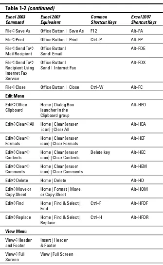
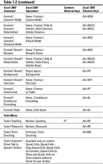
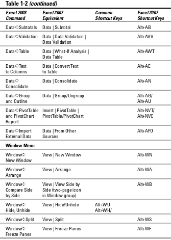
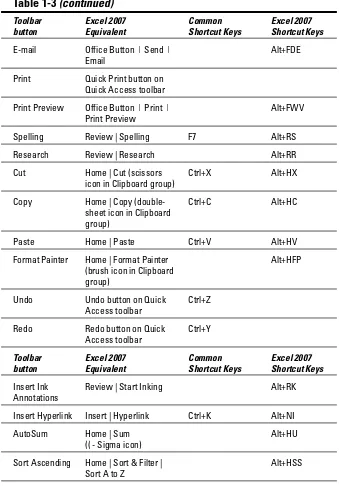
All earlier versions of this book use command arrowsto lead you from the initial pull-down menu, to the submenu, and so on, to the command you ultimately want. For example, if you need to open the File pull-down menu to get to the Open command, that instruction would look like this: Choose File➪Open. This is the equivalent of Office Button | Open and Alt+FO. Commands using the older command arrow notation rather than the vertical bar notation occur only in the tables in Chapter 1 for people upgrading to Excel 2007 from older versions of Excel.
Finally, if you’re really observant, you may notice a discrepancy between the capitalization of the names of dialog box options (such as headings, option buttons, and check boxes) as they appear in text and how they actually appear in Excel on your computer screen. I intentionally use the convention of capitalizing the initial letters of all the main words of a dialog box option to help you differentiate the name of the option from the rest of the text describ-ing its use.
Special icons
The following icons are strategically placed in the margins to point out stuff you may or may not want to read.
This icon alerts you to nerdy discussions that you may well want to skip (or read when no one else is around).
This icon alerts you to shortcuts or other valuable hints related to the topic at hand.
This icon alerts you to information to keep in mind if you want to meet with a modicum of success.
Where to Go from Here
If you’ve never worked with a computer spreadsheet, I suggest that, right after getting your chuckles with the cartoons, you first go to Chapter 1 and find out what you’re dealing with. And, if you’re someone with some experi-ence with earlier versions of Excel, I want you to head directly to the section, “Migrating to Excel 2007 from Earlier Versions” in Chapter 1, where you find out how to stay calm as you become familiar and, yes, comfortable with the new Ribbon user interface.
O
ne look at the Excel 2007 screen with its new Microsoft Office Button, Quick Access toolbar, and Ribbon, and you realize how much stuff is going on here. Well, not to worry: In Chapter 1, I break down the parts of the Excel 2007 Ribbon user interface and make some sense out of the rash of tabs and command buttons that you’re going to be facing day after day after day.The Excel 2007 User Experience
In This Chapter
䊳Getting familiar with the new Excel 2007 program window
䊳Selecting commands from the Ribbon
䊳Customizing the Quick Access Toolbar
䊳Methods for starting Excel 2007
䊳Surfing an Excel 2007 worksheet and workbook
䊳Getting some help with using this program
䊳Quick start guide for users migrating to Excel 2007 from earlier versions
T
he designers and engineers at Microsoft have really gone and done it this time — cooking up a brand new way to use everybody’s favorite electronic spreadsheet program. This new Excel 2007 user interface scraps its previous reliance on a series of pull-down menus, task panes, and multitudinous tool-bars. Instead, it uses a single strip at the top of the worksheet called the Ribbon designed to put the bulk of the Excel commands you use at your fingertips at all times.Add a single remaining Office pull-down menu and sole Quick Access toolbar along with a few remaining task panes (Clipboard, Clip Art, and Research) to the Ribbon and you end up with the easiest to use Excel ever. This version offers you the handiest way to crunch your numbers, produce and print pol-ished financial reports, as well as organize and chart your data, in other words, to do all the wonderful things for which you rely on Excel.
Excel’s Ribbon User Interface
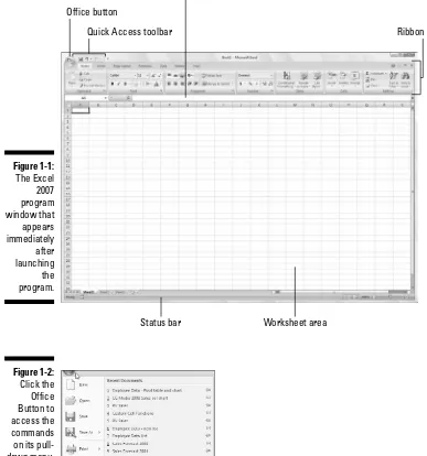
When you first launch Excel 2007, the program opens up the first of three new worksheets (named Sheet1) in a new workbook file (named Book1) inside a program window like the one shown in Figure 1-1 and Color Plate 1.
The Excel program window containing this worksheet of the workbook is made up of the following components:
⻬Office Buttonthat when clicked opens the Office pull-down menu con-taining all the file related commands including Save, Open, Print, and Exit as well as the Excel Options button that enables you to change Excel’s default settings
⻬Quick Access toolbarthat contains buttons you can click to perform common tasks such as saving your work and undoing and redoing edits and which you can customize by adding command buttons
⻬Ribbonthat contains the bulk of the Excel commands arranged into a series of tabs ranging from Home through View
⻬Formula barthat displays the address of the current cell along with the contents of that cell
⻬Worksheet areathat contains all the cells of the current worksheet iden-tified by column headings using letters along the top and row headings using numbers along the left edge with tabs for selecting new worksheets and a horizontal scroll bar to move left and right through the sheet on the bottom and a vertical scroll bar to move up and down through the sheet on the right edge
⻬Status barthat keeps you informed of the program’s current mode, any special keys you engage, and enables you to select a new worksheet view and to zoom in and out on the worksheet
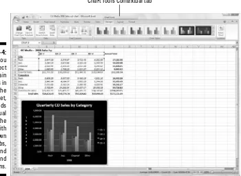
Manipulating the Office Button
At the very top of the Excel 2007 program window, you find the Office Button (the round one with the Office four-color icon in the very upper-left corner of the screen) followed immediately by the Quick Access toolbar.
Figure 1-2:
Click the Office Button to access the commands on its pull-down menu, open a recent workbook, or change the Excel Options.
Quick Access toolbar Ribbon
Office button
Formula bar
Status bar Worksheet area
Figure 1-1:
Bragging about the Ribbon
The Ribbon (shown in Figure 1-3) radically changes the way you work in Excel 2007. Instead of having to memorize (or guess) on which pull-down menu or toolbar Microsoft put the particular command you want to use, their designers and engineers came up with the Ribbon that always shows you all the most commonly used options needed to perform a particular Excel task.
The Ribbon is made up of the following components:
⻬Tabsfor each of Excel’s main tasks that bring together and display all the commands commonly needed to perform that core task
⻬Groupsthat organize related command buttons into subtasks normally performed as part of the tab’s larger core task
⻬Command buttonswithin each group that you select to perform a par-ticular action or to open a gallery from which you can click a parpar-ticular thumbnail — note that many command buttons on certain tabs of the Excel Ribbon are organized into mini-toolbars with related settings
⻬Dialog Box launcherin the lower-right corner of certain groups that opens a dialog box containing a bunch of additional options you can select
To get more of the Worksheet area displayed in the program window, you can minimize the Ribbon so that only its tabs are displayed — simply click Minimize the Ribbon on the menu opened by clicking the Custom Quick Access Toolbar button, double-click any one of the Ribbon’s tabs or press Ctrl+F1. To redisplay the entire Ribbon, and keep all the command buttons on its tab displayed in the program window, click Minimize the Ribbon item on the Custom Quick Access Toolbar’s drop-down menu, double-click one of the tabs or press Ctrl+F1 a second time.
Tabs
Dialog box launcher Groups
Command buttons
Figure 1-3:
When you work in Excel with the Ribbon minimized, the Ribbon expands each time you click one of its tabs to show its command buttons but that tab stays open only until you select one of the command buttons. The moment you select a command button, Excel immediately minimizes the Ribbon again to just the display of its tabs.
Keeping tabs on the Excel Ribbon
The very first time you launch Excel 2007, its Ribbon contains the following seven tabs, going from left to right:
⻬Hometab with the command buttons normally used when creating, formatting, and editing a spreadsheet arranged into the Clipboard, Font, Alignment, Number, Styles, Cells, and Editing groups (see Color Plate 1)
⻬Inserttab with the command buttons normally used when adding par-ticular elements (including graphics, PivotTables, charts, hyperlinks, and headers and footers) to a spreadsheet arranged into the Shapes, Tables, Illustrations, Charts, Links, and Text groups (see Color Plate 2)
⻬Page Layouttab with the command buttons normally used when pre-paring a spreadsheet for printing or re-ordering graphics on the sheet arranged into the Themes, Page Setup, Scale to Fit, Sheet Options, and Arrange groups (see Color Plate 3)
⻬Formulastab with the command buttons normally used when adding formulas and functions to a spreadsheet or checking a worksheet for for-mula errors arranged into the Function Library, Defined Names, Forfor-mula Auditing, and Calculation groups (see Color Plate 4). Note that this tab also contains a Solutions group when you activate certain add-in programs such as Conditional Sum and Euro Currency Tools — see Chapter 12 for more on using Excel add-in programs.
⻬Datatab with the command buttons normally used when importing, querying, outlining, and subtotaling the data placed into a worksheet’s data list arranged into the Get External Data, Manage Connections, Sort & Filter, Data Tools, and Outline groups (see Color Plate 5). Note that this tab also contains an Analysis group if you activate add-ins such as the Analysis Toolpak and Solver Add-In — see Chapter 12 for more on Excel add-ins.
⻬Reviewtab with the command buttons normally used when proofing, protecting, and marking up a spreadsheet for review by others arranged into the Proofing, Comments, and Changes, groups (see Color Plate 6). Note that this tab also contains an Ink group with a sole Start Inking button if you’re running Office 2007 on a Tablet PC.
In addition to these seven standard tabs, Excel has an eighth, optional Developer tab that you can add to the Ribbon if you do a lot of work with macros and XML files — see Chapter 12 for more on the Developer tab.
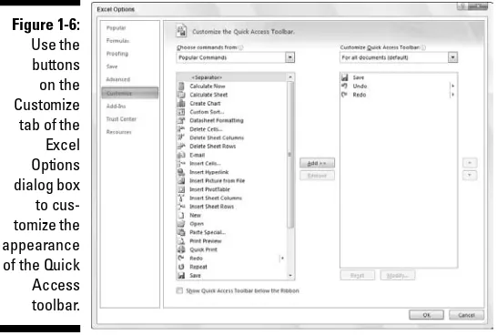
Although these standard tabs are the ones you always see on the Ribbon when it’s displayed in Excel, they aren’t the only things that can appear in this area. In addition, Excel can display contextual tools when you’re working with a particular object that you select in the worksheet such as a graphic image you’ve added or a chart or PivotTable you’ve created. The name of the contextual tools for the selected object appears immediately above the tab or tabs associated with the tools.
For example, Figure 1-4 shows a worksheet after you click the embedded chart to select it. As you can see, doing this causes the contextual tool called Chart Tools to be added to the very end of the Ribbon. Chart Tools contex-tual tool has its own three tabs: Design (selected by default), Layout, and Format. Note too that the command buttons on the Design tab are arranged into their own groups: Type, Data, Chart Layouts, Chart Styles, and Location.
The moment you deselect the object (usually by clicking somewhere on the sheet outside of its boundaries), the contextual tool for that object and all of its tabs immediately disappears from the Ribbon, leaving only the regular tabs — Home, Insert, Page Layout, Formulas, Data, Review, and View — displayed.
Chart Tools Contextual tab
Figure 1-4:
Selecting commands from the Ribbon
The most direct method for selecting commands on the Ribbon is to click the tab that contains the command button you want and then click that button in its group. For example, to insert a piece of Clip Art into your spreadsheet, you click the Insert tab and then click the Clip Art button to open the Clip Art task pane in the Worksheet area.
The easiest method for selecting commands on the Ribbon — if you know your keyboard at all well — is to press the Alt key and then type the sequence of letters designated as the hot keys for the desired tab and associated command buttons.
When you first press and release the Alt key, Excel displays the hot keys for all the tabs on the Ribbon. When you type one of the Ribbon tab hot keys to select it, all the command button hot keys appear next to their buttons along with the hot keys for the Dialog Box launchers in any group on that tab (see Figure 1-5). To select a command button or Dialog Box launcher, simply type its hot key letter.
If you know the old Excel shortcut keys from versions Excel 97 through 2003, you can still use them. For example, instead of going through the rigmarole of pressing Alt+HC to copy a cell selection to the Windows Clipboard and then Alt+HV to paste it elsewhere in the sheet, you can still press Ctrl+C to copy the selection and then press Ctrl+V when you’re ready to paste it. Note, how-ever, that when using a hot key combination with the Alt key, you don’t need to keep the Alt key depressed while typing the remaining letter(s) as you do when using a hot key combo with the Ctrl key.
Figure 1-5:
Adapting the Quick Access toolbar
When you first start using Excel 2007, the Quick Access toolbar contains only the following few buttons:
⻬Saveto save any changes made to the current workbook using the same filename, file format, and location
⻬Undoto undo the last editing, formatting, or layout change you made ⻬Redoto reapply the previous editing, formatting, or layout change that
you just removed with the Undo button
The Quick Access toolbar is very customizable as Excel makes it really easy to add any Ribbon command to it. Moreover, you’re not restricted to adding buttons for just the commands on the Ribbon: you can add any Excel com-mand you want to the toolbar, even the obscure ones that don’t rate an appearance on any of its tabs.
By default, the Quick Access toolbar appears above the Ribbon tabs immedi-ately to the right of the Office Button. To display the toolbar beneath the Ribbon immediately above the Formula bar, click the Customize Quick Access Toolbar button (the drop-down button to the right of the toolbar with a horizontal bar above a down-pointing triangle) and then click Show Below the Ribbon on its drop-down menu. You will definitely want to make this change if you start adding more buttons to the toolbar so that the grow-ing Quick Access toolbar doesn’t start crowdgrow-ing out the name of the current workbook that appears to the toolbar’s right.
Adding command buttons on the Customize
Quick Access Toolbar’s drop-down menu
When you click the Customize Quick Access Toolbar button, a drop-down menu appears containing the following commands:
⻬Newto open a new workbook
⻬Opento display the Open dialog box for opening an existing workbook ⻬Saveto save changes to your current workbook
⻬E-mailto open your mail
⻬Quick Printto send the current worksheet to your default printer ⻬Print Previewto open the current worksheet in the Print Preview window ⻬Spellingto check the current worksheet for spelling errors
⻬Redoto reapply the last edit that you removed with Undo
⻬Sort Ascendingto sort the current cell selection or column in A to Z alphabetical, lowest to highest numerical, or oldest to newest date order
⻬Sort Descendingto sort the current cell selection or column Z to A alphabetical, highest to lowest numerical, or newest to oldest date order
When you first open this menu, only the Save, Undo, and Redo options are selected (indicated by the check marks in front of their names) and therefore theirs are the only buttons to appear on the Quick Access toolbar. To add any of the other commands on this menu to the toolbar, you simply click the option on the drop-down menu. Excel then adds a button for that command to the end of the Quick Access toolbar (and a check mark to its option on the drop-down menu).
To remove a command button that you add to the Quick Access toolbar in this manner, click the option a second time on the Customize Quick Access Toolbar button’s drop-down menu. Excel removes its command button from the toolbar and the check mark from its option on the drop-down menu.
Adding command buttons on the Ribbon
To add any Ribbon command to the Quick Access toolbar, simply right-click its command button on the Ribbon and then click Add to Quick Access Toolbar on its shortcut menu. Excel then immediately adds the command button to the very end of the Quick Access toolbar, immediately in front of the Customize Quick Access Toolbar button.
If you want to move the command button to a new location on the Quick Access toolbar or group with other buttons on the toolbar, you need to click the Customize Quick Access Toolbar button and then click the More
Commands option near the bottom of its drop-down menu.
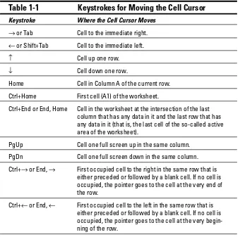
Excel then opens the Excel Options dialog box with the Customize tab selected (similar to the one shown in Figure 1-6). Here, Excel shows all the buttons currently added to the Quick Access toolbar with the order in which they appear from left to right on the toolbar corresponding to their top-down order in the list box on the right-hand side of the dialog box.
You can add separators to the toolbar to group related buttons. To do this, click the <Separator> selection in the list box on the left and then click the Add button twice to add two. Then, click the Move Up or Move Down buttons to position one of the two separators at the beginning of the group and the other at the end.
To remove a button added from the Ribbon, right-click it on the Quick Access toolbar and then click the Remove from Quick Access Toolbar option on its shortcut menu.
Adding non-Ribbon commands to the Quick Access toolbar
You can also use the options on the Customize tab of the Excel Options dialog box (see Figure 1-6) to add a button for any Excel command even if it’s is not one of those displayed on the tabs of the Ribbon:1. Click the type of command you want to add to the Quick Access tool-bar in the Choose Commands From drop-down list box.
The types of commands include the File pull-down menu (the default) as well as each of the tabs that appear on the Ribbon. To display only the commands that are not displayed on the Ribbon, click Commands Not in the Ribbon near the bottom of the drop-down list. To display a complete list of all the Excel commands, click All Commands at the very bottom of the drop-down list.
2. Click the command whose button you want to add to the Quick Access toolbar in the list box on the left.
Figure 1-6:
3. Click the Add button to add the command button to the bottom of the list box on the right.
4. (Optional) To reposition the newly added command button so that it’s not the last one on the toolbar, click the Move Up button until it’s in the desired position.
5. Click the OK button to close Excel Options dialog box.
If you’ve created favorite macros (see Chapter 12) that you routinely use and want to be able to run directly from the Quick Access toolbar, click Macros in the Choose Commands From drop-down list box in the Excel Options dialog box and then click the name of the macro to add followed by the Add button.
Having fun with the Formula bar
The Formula bar displays the cell address and the contents of the current cell. The address of this cell is determined by its column letter(s) followed immediately by the row number as in cell A1, the very first cell of each work-sheet at the intersection of column A and row 1 or cell XFD1048576, the very last of each Excel 2007 worksheet, at the intersection of column XFD and row 1048576. The contents of the current cell are determined by the type of entry you make there: text or numbers if you just enter a heading or particular value and the nuts and bolts of a formula if you enter a calculation there.
The Formula bar is divided into three sections:
⻬Name box:The left-most section that displays the address of the current cell address
⻬Formula bar buttons:The second, middle section that appears as a rather nondescript button displaying only an indented circle on the left (used to narrow or widen the Name box) with the Function Wizard button (labeled fx) on the right until you start making or editing a cell entry at which time, its Cancel (an X) and its Enter (a check mark) but-tons appear in between them
⻬Cell contents:The third, right-most white area to the immediate right of the Function Wizard button that takes up the rest of the bar and expands as necessary to display really, really long cell entries that won’t fit the normal area
What to do in the Worksheet area
The Worksheet area is where most of the Excel spreadsheet action takes place because it’s the place that displays the cells in different sections of the current worksheet and it’s right inside the cells that you do all your spread-sheet data entry and formatting, not to mention a great deal of your editing.
Keep in mind that in order for you to be able to enter or edit data in a cell, that cell must be current. Excel indicates that a cell is current in three ways:
⻬The cell cursor — the dark black border surrounding the cell’s entire perimeter — appears in the cell
⻬The address of the cell appears in the Name box of the Formula bar
⻬The cell’s column letter(s) and row number are shaded (in a kind of a beige color on most monitors) in the column headings and row headings that appear at the top and left of the Worksheet area, respectively
Moving around the worksheet
An Excel worksheet contains far too many columns and rows for all of a worksheet’s cells to be displayed at one time regardless of how large your personal computer monitor screen is or how high the screen resolution. (After all, we’re talking 17,179,869,184 cells total!) Excel therefore offers many methods for moving the cell cursor around the worksheet to the cell where you want to enter new data or edit existing data:
⻬Click the desired cell — assuming that the cell is displayed within the section of the sheet currently visible in the Worksheet area
Click the Name box, type the address of the desired cell directly into this box and then press the Enter key
How you assign 26 letters to 16,384 columns
When it comes to labeling the 16,384 columns of an Excel 2007 worksheet, our alphabet with its measly 26 letters is simply not up to the task. To make up the difference, Excel first doubles the letters in the cell’s column reference so that column AA follows column Z (after which you find column AB, AC, and so on) and then triples
⻬Press F5 to open the Go To dialog box, type the address of the desired cell into its Reference text box and then click OK
⻬Use the cursor keys as shown in Table 1-1 to move the cell cursor to the desired cell
⻬Use the horizontal and vertical scroll bars at the bottom and right edge of the Worksheet area to move the part of the worksheet that contains the desired cell and then click the cell to put the cell cursor in it
Keystroke shortcuts for moving the cell cursor
Excel offers a wide variety of keystrokes for moving the cell cursor to a new cell. When you use one of these keystrokes, the program automatically scrolls a new part of the worksheet into view, if this is required to move the cell pointer. In Table 1-1, I summarize these keystrokes and how far each one moves the cell pointer from its starting position.
Table 1-1
Keystrokes for Moving the Cell Cursor
Keystroke Where the Cell Cursor Moves
→or Tab Cell to the immediate right.
←or Shift+Tab Cell to the immediate left.
↑ Cell up one row.
↓ Cell down one row.
Home Cell in Column A of the current row.
Ctrl+Home First cell (A1) of the worksheet.
Ctrl+End or End, Home Cell in the worksheet at the intersection of the last column that has any data in it and the last row that has any data in it (that is, the last cell of the so-called active area of the worksheet).
PgUp Cell one full screen up in the same column.
PgDn Cell one full screen down in the same column.
Ctrl+→or End, → First occupied cell to the right in the same row that is either preceded or followed by a blank cell. If no cell is occupied, the pointer goes to the cell at the very end of the row.
Ctrl+←or End, ← First occupied cell to the left in the same row that is either preceded or followed by a blank cell. If no cell is occupied, the pointer goes to the cell at the very begin-ning of the row.
Table 1-1 (continued)
Keystroke Where the Cell Cursor Moves
Ctrl+↑or End, ↑ First occupied cell above in the same column that is either preceded or followed by a blank cell. If no cell is occupied, the pointer goes to the cell at the very top of the column.
Ctrl+↓or End, ↓ First occupied cell below in the same column that is either preceded or followed by a blank cell. If no cell is occupied, the pointer goes to the cell at the very bottom of the column.
Ctrl+Page Down Last occupied cell in the next worksheet of that workbook.
Ctrl+Page Up Last occupied cell in the previous worksheet of that workbook.
Note:In the case of those keystrokes that use arrow keys, you must either use the arrows on the cursor keypad or else have the Num Lock disengaged on the numeric keypad of your keyboard.
The keystrokes that combine the Ctrl or End key with an arrow key listed in Table 1-1 are among the most helpful for moving quickly from one edge to the other in large tables of cell entries or in moving from table to table in a sec-tion of the worksheet that contains many blocks of cells.
When you use Ctrl and an arrow key to move from edge to edge in a table or between tables in a worksheet, you hold down Ctrl while you press one of the four arrow keys (indicated by the +symbol in keystrokes, such as Ctrl+→). When you use End and an arrow-key alternative, you must press and then release the End key beforeyou press the arrow key (indicated by the comma in keystrokes, such as End, →). Pressing and releasing the End key causes the End Mode indicator to appear on the status bar. This is your sign that Excel is ready for you to press one of the four arrow keys.
Because you can keep the Ctrl key depressed as you press the different arrow keys that you need to use, the Ctrl-plus-arrow-key method provides a more fluid method for navigating blocks of cells than the End-then-arrow-key method.
After engaging Scroll Lock, when you scroll the worksheet with the keyboard, Excel does not select a new cell while it brings a new section of the work-sheet into view. To “unfreeze” the cell pointer when scrolling the workwork-sheet via the keyboard, you just press the Scroll Lock key again.
Tips on using the scroll bars
To understand how scrolling works in Excel, imagine its humongous work-sheet as a papyrus scroll attached to rollers on the left and right. To bring into view a new section of a papyrus worksheet that is hidden on the right, you crank the left roller until the section with the cells that you want to see appears. Likewise, to scroll into view a new section of the worksheet that is hidden on the left, you would crank the right roller until that section of cells appears.
You can use the horizontal scroll bar at the bottom of the Worksheet area to scroll back and forth through the columns of a worksheet and the vertical scroll bar to scroll up and down through its rows. To scroll a column or a row at a time in a particular direction, click the appropriate scroll arrow at the ends of the scroll bar. To jump immediately back to the originally displayed area of the worksheet after scrolling through single columns or rows in this fashion, simply click the black area in the scroll bar that now appears in front of or after the scroll bar.
Keep in mind that you can resize the horizontal scroll bar making it wider or narrower by dragging the button that appears to the immediate left of its left scroll arrow. Just keep in mind when working in a workbook that contains a whole bunch of worksheets that in widening the horizontal scroll bar you can end up hiding the display of the workbook’s later sheet tabs.
To scroll very quickly through columns or rows of the worksheet, hold down the Shift key and then drag the mouse pointer in the appropriate direction within the scroll bar until the columns or rows that you want to see appear on the screen in the Worksheet area. When you hold down the Shift key as you scroll, the scroll button within the scroll bar becomes real skinny and a ScreenTip appears next to the scroll bar, keeping you informed of the letter(s) of the columns or the numbers of the rows that you’re currently whizzing through.
The only disadvantage to using the scroll bars to move around is that the scroll bars bring only new sections of the worksheet into view — they don’t actually change the position of the cell cursor. If you want to start making entries in the cells in a new area of the worksheet, you still have to remember to select the cell (by clicking it) or the group of cells (by dragging through them) where you want the data to appear before you begin entering the data.
Surfing the sheets in a workbook
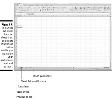
Each new workbook you open in Excel 2007 contains three blank worksheets, each with its own 16,384 columns and 1,048,576 rows (giving you a truly stag-gering total of 51,539,607,552 blank cells!). But that’s not all, if ever you need more worksheets in your workbook; you can add them simply by clicking the Insert Worksheet button that appears to the immediate right of the last sheet tab (see Figure 1-7).
First sheet
Previous sheet
Next sheet Last sheet
Sheet Tab scroll buttons
Insert Worksheet
Figure 1-7:
On the left side of the bottom of the Worksheet area, the Sheet Tab scroll but-tons appear followed by the actual tabs for the worksheets in your workbook and the Insert Worksheet button. To activate a worksheet for editing, you select it by clicking its sheet tab. Excel lets you know what sheet is active by displaying the sheet name in boldface type and making its tab appear on top of the others.
Don’t forget the Ctrl+Page Down and Ctrl+Page Up shortcut keys for selecting the next and previous sheet, respectively, in your workbook.
If your workbook contains too many sheets for all their tabs to be displayed at the bottom of the Worksheet area, use the Sheet Tab scroll buttons to bring new tabs into view (so that you can then click them to activate them). You click the Next Sheet button to scroll the next hidden sheet tab into view or the Last Sheet button to scroll the last group of completely or partially hidden tabs into view.
Showing off the Status bar
The Status bar is the last component at the very bottom of the Excel program window (see Figure 1-8). The Status bar contains the following areas:
⻬Modebutton that indicates the current state of the Excel program (Ready, Edit, and so on) as well as any special keys that are engaged (Caps Lock, Num Lock, and Scroll Lock)
⻬Macro Recordingbutton (the red dot) that opens the Record Macro dialog box where you can set the parameters for a new macro and begin recording it (see Chapter 12)
One reason for adding extra sheets to a workbook
You may wonder why on earth anyone would ever need more than three worksheets given just how many cells each individual sheet contains. The simple truth is that it’s all about how you choose to structure a particular spreadsheet rather than running out of places to put the data. For example, suppose that you need to create a workbook that contains budgets for all the vari-ous departments in your corporation, you may decide to devote an individual worksheet to each
⻬AutoCalculateindicator that displays the Average and Sum of all the numerical entries in the current cell selection along with the Count of every cell in selection
⻬Layoutselector that enables you to select between three layouts for the Worksheet area: Normal, the default view that shows only the worksheet cells with the column and row headings; Page Layout View that adds rulers, page margins, and shows page breaks for the worksheet; and Page Break Preview that enables you to adjust the paging of a report (see Chapter 5 for details)
⻬Zoomslider that enables you to zoom in and out on the cells in the Worksheet area by dragging the slider to the right or left, respectively
The Num Lock indicator tells you that you can use the numbers on the numeric keypad for entering values in the worksheet. This keypad will most often be separate from the regular keyboard on the right side if you’re using a separate keyboard and embedded in keys on the right side of the regular key-board on almost all laptop computers where the keykey-board is built right into the computer.
Mode Indicator
Auto Calculate Indicator Layout Selector
Zoom slider
Record Macro
Figure 1-8:
Starting and Exiting Excel
Excel 2007 runs under both the older Windows XP operating system and the brand new Windows Vista operating system. Because of changes made to the Start menu in Windows Vista, the procedure for starting Excel from this version of Windows is a bit different from Windows XP.
Starting Excel from the Windows
Vista Start menu
You can use the Start Search box at the bottom of the Windows Vista Start menu to locate Excel on your computer and launch the program in no time at all:
1. Click the Start button on the Windows taskbar to open the Windows Start menu.
2. Click the Start Search text box and type the two letters exto have Vista locate Microsoft Office Excel 2007 on your computer.
3. Click the Microsoft Office Excel 2007 option that now appears in the left Programs column on the Start menu.
If you have more time on your hands, you can also launch Excel from the Vista Start menu by going through the rigmarole of clicking Start➪ All Programs➪Microsoft Office➪Microsoft Office Excel 2007.
Starting Excel from the Windows
XP Start menu
When starting Excel 2007 from the Windows XP Start menu, you follow these simple steps:
1. Click the Start button on the Windows taskbar to open the Windows Start menu.
Pinning Excel to the Start menu
If you use Excel all the time, you may want to make its program option a per-manent part of the Windows Start menu. To do this, you pin the program option to the Start menu (and the steps for doing this are the same in Windows XP as they are in Windows Vista):
1. Start Excel from the Windows Start menu.
In launching Excel, use the appropriate method for your version of Windows as outlined in the “Starting Excel from the Windows Vista Start menu” or the “Starting Excel from the Windows XP Start menu” section earlier in this chapter.
After launching Excel, Windows adds Microsoft Office 2007 to the recently used portion on the left side of the Windows Start menu.
2. Click the Start menu and then right-click Microsoft Excel 2007 on the Start menu to open its shortcut menu.
3. Click Pin to Start menu on the shortcut menu.
After pinning Excel in this manner, the Microsoft Office Excel 2007 option always appears in the upper section of the left-hand column of the Start menu and you can then launch Excel simply by clicking the Start button and then click this option.
Creating an Excel desktop shortcut
for Windows Vista
Some people prefer having the Excel Program icon appear on the Windows desktop so that they can launch the program from the desktop by double-clicking this program icon. To create an Excel program shortcut for Windows Vista, you follow these steps:
1. Click the Start button on the Windows taskbar.
The Start menu opens where you click the Start Search text box.
2. Click the Start Search text box and type excel.exe.
3. Right-click the file icon for the excel.exefile at the top of the Start
menu and then highlight Send To on the pop-up menu and click Desktop (Create Shortcut) on its continuation menu.
A shortcut named EXCEL -Shortcut appears to your desktop. You should probably rename the shortcut to something a little more friendly, such as Excel 2007.
4. Right-click the EXCEL - Shortcut icon on the Vista desktop and then click Rename on the pop-up menu.
5. Replace the current name by typing a new shortcut name, such as
Excel 2007 and then click anywhere on the desktop.
Creating an Excel desktop
shortcut for Windows XP
If you’re running Excel 2007 on Windows XP, you use the following steps to create a program shortcut for your Windows XP desktop:
1. Click the Start button on the Windows taskbar.
The Start menu opens the Search item.
2. Click Search in the lower-right corner of the Start menu.
The Search Results dialog box appears.
3. Click the All Files and Folders link in the panel on the left side of the Search Results dialog box.
The Search Companion pane appears on the left side of the Search Results dialog box.
4. Type excel.exe in the All or Part of the File Name text box.
Excel.exeis the name of the executable program file that runs Excel. After finding this file on your hard disk, you can create a desktop short-cut from it that launches the program.
5. Click the Search button.
Windows now searches your hard disk for the Excel program file. After locating this file, its name appears on the right side of the Search Results dialog box. When this filename appears, you can click the Stop button in the left panel to halt the search.
6. Right-click the file icon for the excel.exefile and then highlight
Send To on the pop-up menu and click Desktop (Create Shortcut) on its continuation menu.
7. Click the Close button in the upper-right corner of the Search Results dialog box.
After closing the Search Results dialog box, you should see the icon named Shortcut to excel.exe on the desktop. You should probably rename the shortcut to something a little more friendly, such as Excel 2007.
8. Right-click the Shortcut to excel.exe icon and then click Rename on the pop-up menu.
9. Replace the current name by typing a new shortcut name, such as
Excel 2007 and then click anywhere on the desktop.
After you create an Excel desktop shortcut on the Windows XP desktop you can launch Excel by double-clicking the shortcut icon.
Adding the Excel desktop shortcut
to the Quick Launch toolbar
If you want to be able to launch Excel 2007 by clicking a single button, drag the icon for your Excel Windows Vista or XP desktop shortcut to the Quick Launch toolbar to the immediate right of the Start button at the beginning of the Windows taskbar. When you position the icon on this toolbar, Windows indicates where the new Excel button will appear by drawing a black, vertical I-beam in front of or between the existing buttons on this bar. As soon as you release the mouse button, Windows adds an Excel 2007 button to the Quick Launch toolbar that enables you to launch the program by a single-click of its icon.
Exiting Excel
When you’re ready to call it a day and quit Excel, you have several choices for shutting down the program:
⻬Click the Office Button followed by the Exit Excel button
⻬Press Alt+FX or Alt+F4
⻬Click the Close button in the upper-right corner of the Excel program window (the X)